Data exploration

Incidence data

Let’s get the dengue data:

dengue <- readr::read_csv("https://raw.githubusercontent.com/choisy/DMo2019/master/data/dengue.csv")

You can split the data frame of incidences into a list of data frames, with one data frame per state as so:

dengue_by_state <- split(dengue, dengue$state)

From which list you can extract whatever state you want:

dengue_data <- dengue_by_state$Terengganu

Let’s define some coordinates to customize the $x$-axis:

ats <- dengue_data %>%
  dplyr::group_by(year) %>%
  dplyr::summarise(at = mean(week)) %>%
  dplyr::ungroup() %$%
  setNames(at, year) 

and

first_weeks <- which(dengue_data$week == 1) - .5

The following function plots a chronologically-order vector of incidence from the list dengue_by_state:

plot_incidence <- function(x, ...) {
  barplot(x, space = 0, axes = FALSE, xlab = NA, ylab = "incidence", ...)
  axis(1, first_weeks, FALSE)
  axis(1, ats + first_weeks, names(ats), tick = FALSE)
  axis(2)
  abline(v = first_weeks, lty = 2, col = "grey")
}

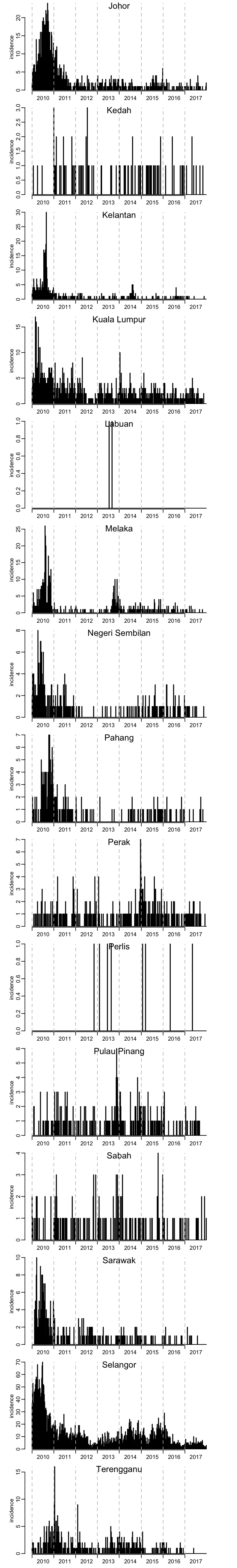
Let’s use this function to plot the time series of incidence for all the states:

par(mfrow = c(15, 1))
for (state in unique(dengue$state)) {
  plot_incidence(dengue_by_state[[state]]$incidence)
  mtext(state, line = -1)
}

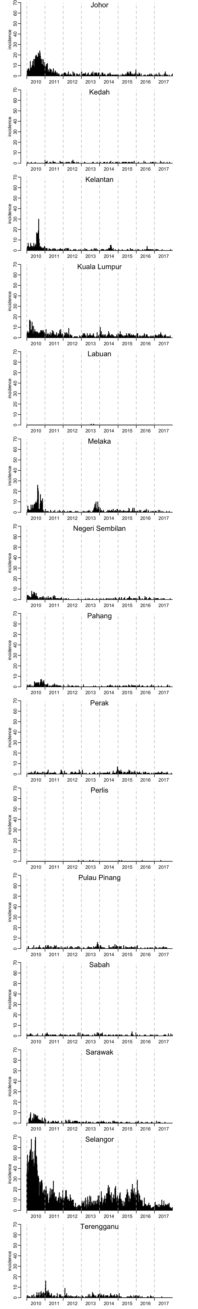
The same, but this time with the same range of values on the $y$-axis:

par(mfrow = c(15, 1))
for (state in unique(dengue$state)) {
  plot_incidence(dengue_by_state[[state]]$incidence, ylim = c(0, max(dengue$incidence)))
  mtext(state, line = -1)
}

Geographic data

We can download maps of any country directly from the GADM website:

malaysia <- readRDS(url("https://biogeo.ucdavis.edu/data/gadm3.6/Rsf/gadm36_MYS_1_sf.rds"))

Climatic data

Downloading the climatic stations:

stations <- readr::read_csv("https://raw.githubusercontent.com/choisy/DMo2019/master/data/climatic%20stations.csv")

Plotting the locations of the climatic stations. First we need to transform the stations as a geographic object:

stations_geo <- sf::st_as_sf(stations,
                             coords = c("longitude", "latitude"),
                             crs = "+proj=longlat +datum=WGS84 +no_defs +ellps=WGS84 +towgs84=0,0,0")

malaysia %>%
  sf::st_simplify(TRUE, .05) %>% 
  sf::st_geometry() %>% 
  plot(col = "lightgrey")
plot(stations_geo, add = TRUE, pch = 3, col = "red")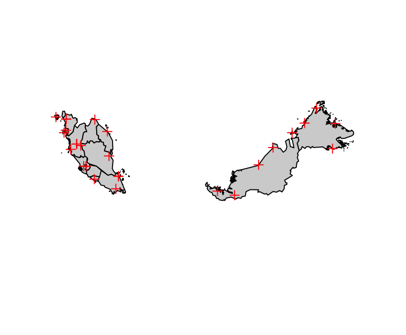

Let’s now download the climatic data:

climate <- readr::read_csv("https://raw.githubusercontent.com/choisy/DMo2019/master/data/climate.csv")

Let’s now aggregate these data by epi week so that we can compare more easily with the incidence data that are also defined by epi week:

climate_week <- climate %>%
  dplyr::mutate(year = lubridate::year(day),
                week = lubridate::epiweek(day)) %>% 
  dplyr::select(-day) %>% 
  dplyr::group_by(station, year, week) %>%
  dplyr::summarise_all(mean, na.rm = TRUE) %>% 
  dplyr::ungroup() %>% 
  dplyr::mutate_at(dplyr::vars(ra, sn, ts, fg), list(~ . > 0)) %>% 
  dplyr::mutate_all(. %>% ifelse(is.nan(.), NA, .))

Relating climatic data to incidence data

Let’s say that we want to focus on the state of Selangor and we want to identify the climatic stations that are in this state:

selangor <- dplyr::filter(malaysia, NAME_1 == "Selangor")
selangor_station <- stations_geo[as.integer(sf::st_contains(selangor, stations_geo)), ]

Let’s see that on the map:

plot(sf::st_geometry(selangor), col = "lightgrey")
plot(stations_geo, add = TRUE, pch = 3, col = "red")
plot(selangor_station, add = TRUE, col = "blue")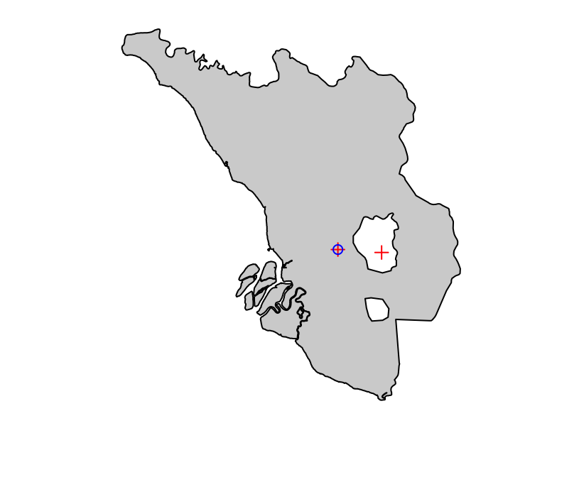

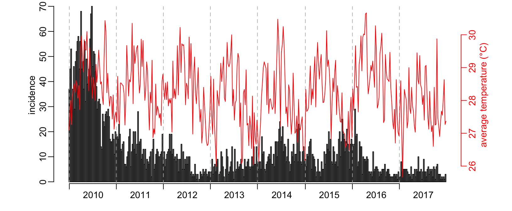
Now we can compare incidence with for example average temperature for the state of Selangor:

plot_incidence(dengue_by_state$Selangor$incidence)
par(new = TRUE)
climate_week %>%
  dplyr::filter(station == selangor_station$station) %>%
  dplyr::arrange(year, week) %$%
  plot(ta, type = "l", col = "red", axes = FALSE, ann = FALSE)
axis(4, col = "red", col.axis = "red")
mtext("average temperature (°C)", 4, 1.5, col = "red")