Logistic classification

Parameters

The path to the data folder:

data_path <- paste0("/Users/MarcChoisy/Library/CloudStorage/",
                    "OneDrive-OxfordUniversityClinicalResearchUnit/",
                    "GitHub/choisy/typhoid/")

Reading the clean data

The path to the data:

nepal <- readRDS(paste0(data_path, "clean_data/nepal.rds"))

Packages

required packages:

required_packages <- c("dplyr", "purrr", "rsample", "parsnip", "probably", "magrittr",
                       "yardstick", "tidyr")

Making sure that the required packages are installed:

to_inst <- required_packages[! required_packages %in% installed.packages()[,"Package"]]
if (length(to_inst)) install.packages(to_inst)

Loading some of these packages:

library(dplyr)
library(purrr)
library(rsample)
library(parsnip)
library(recipes)
library(workflows)
library(probably)
library(tune)
library(yardstick)

Feature engineering

Nepal data set:

nepal2 <- nepal |> 
  mutate(across(c(Cough, Diarrhoea, vomiting, Abdopain, Constipation, Headache,
                  Anorexia, Nausea, Typhoid_IgM), ~ .x > 0),
         across(`CRP_mg/L`, ~ .x != "<10"),
         across(Fever, ~ .x > 4),
         across(OralTemperature, ~ .x >= 39),
         `pulse<100` = Pulse < 100,
         `pulse>120` = Pulse > 120,
         across(where(is.logical), as.factor)) |> 
  select(BloodCSResult, Sex, Age, contains("core"), where(is.logical), everything())

A classifier based on logistic regression

A logistic regression model

Let’s start with a simple example where we consider only the symptom variables:

nepal3 <- nepal2[, c(1, 9:17)]

Let’s create the train and test data sets:

data_split <- initial_split(nepal3)
train_data <- training(data_split)
test_data <- testing(data_split)

Defining the logistic regression:

model <- logistic_reg() |> 
  set_engine("glm")

The formula of the classifier:

recette <- recipe(BloodCSResult ~ ., data = train_data)

Let’s put the logistic regression and the formula together:

wflow <- workflow() |> 
  add_recipe(recette) |> 
  add_model(model)

Making and training a classifier

So far with have a logistic regression model. It can be used as such as a classifier, in which case it will by default assign TRUE to a probability above 0.5 and FALSE otherwise. But maybe this 0.5 probability threshold is not the optimal value for the classification task. This threshold can be considered as a hyper-parameter to be tuned. Here is the task is quite easy since there is only one hyper-parameter and that this hyper-parameter is constrained to be between 0 and 1. We can thus do an exhaustive search. To do so we will do a 10-fold cross validation scheme to make sure that the value of the hyper-parameter is assessed on unseen data.

folds <- vfold_cv(train_data)

The following function fit the logistic regression on the training set of a given fold and then compute the performance metrics for threshold values varying between epsilon and 1 - epsilon by step of epsilon on the evaluation set of the fold.

compute_metrics2 <- function(fold, epsilon = .01) {
  thresholds <- seq(epsilon, 1 - epsilon, epsilon)
  validate_data <- testing(get_rsplit(folds, fold))
  
  fit(wflow, data = training(get_rsplit(folds, fold))) |> 
    predict(validate_data, type = "prob") |>
    bind_cols(validate_data) |> 
    threshold_perf(BloodCSResult, .pred_FALSE, thresholds) |> 
    mutate(fold = fold)
}

Calling this function for the folds and gathering the output in a data frame:

the_metrics <- folds |> 
  nrow() |> 
  seq_len() |>
  map_dfr(compute_metrics2)

Computing the mean of the metrics across the folds:

the_metrics2 <- the_metrics |> 
  group_by(.threshold, .metric) |> 
  summarise(estimate = mean(.estimate)) |> 
  ungroup()

`summarise()` has grouped output by '.threshold'. You can override using the
`.groups` argument.

Displaying the metrics and the optimal value of the hyper-parameter:

lwd_val <- 4
lines2 <- function(...) lines(..., lwd = lwd_val)
plot2 <- function(...) plot(..., asp = 1, xaxs = "i", yaxs = "i")

opar <- par(pty = "s", mfrow = 1:2)

# Left panel:
the_metrics |> 
  filter(.metric == "sensitivity") |> 
  with(plot2(.threshold, .estimate, col = 4,
             xlab = "probability threshold", ylab = "metric"))

the_metrics |> 
  filter(.metric == "specificity") |> 
  with(points(.threshold, .estimate, col = 2))

the_metrics |> 
  filter(.metric == "j_index") |> 
  with(points(.threshold, .estimate, col = 3))

the_metrics2 |> 
  filter(.metric == "sensitivity") |> 
  with(lines2(.threshold, estimate, col = 4))

the_metrics2 |> 
  filter(.metric == "specificity") |> 
  with(lines2(.threshold, estimate, col = 2))

the_metrics2 |> 
  filter(.metric == "j_index") |> 
  with(lines2(.threshold, estimate, col = 3))

tuned_threshold <- the_metrics2 |> 
  filter(.metric == "j_index") |> 
  filter(estimate == max(estimate)) |> 
  pull(.threshold)

abline(v = tuned_threshold, lwd = lwd_val)

legend("left", legend = c("sensitivity", "specificity", "j index"),
       col = c(2, 4, 3), lwd = lwd_val, bty = "n")
box(bty = "o")

# ROC curve:
opar <- par(pty = "s")

the_metrics3 <- the_metrics2 |> 
  filter(.metric != "j_index") |> 
  tidyr::pivot_wider(names_from = .metric, values_from = estimate)

with(the_metrics3, plot2(1 - specificity, sensitivity, type = "l", lwd = lwd_val))

abline(0, 1)
box(bty = "o")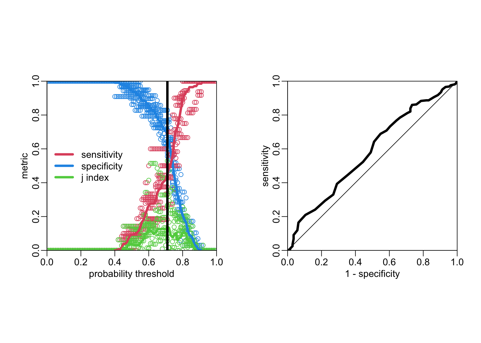

par(opar)

The tuned hyper-parameter value is

tuned_threshold

[1] 0.71

The value of the AUC is:

.5 + with(the_metrics3, sum(.01 * (sensitivity + specificity - 1)))

[1] 0.5324543

Testing the classifier on the test data set:

Preparing the data to evaluate:

to_evaluate <- wflow |>
  fit(data = train_data) |> 
  predict(test_data, type = "prob") |>
  mutate(predictions = make_two_class_pred(.pred_FALSE, c("FALSE", "TRUE"),
                                           tuned_threshold)) |> 
  bind_cols(test_data)

Let’s evaluate:

conf_mat(to_evaluate, BloodCSResult, predictions)

          Truth
Prediction FALSE TRUE
     FALSE    72   17
     TRUE     35   26

metric_set(sens, spec)(to_evaluate, BloodCSResult, estimate = predictions)

# A tibble: 2 × 3
  .metric .estimator .estimate
  <chr>   <chr>          <dbl>
1 sens    binary         0.673
2 spec    binary         0.605