ref_conc <- 10Processing tetanus ELISA data
Warning: Anti_toxin was missing on the cell 68F of the tab Plate_22_hcdc.
1 Parameters
The concentration of the reference anti-toxin is 10 IU/mL:
The threshold for positivity (in IU/mL):
positive_threshold <- .1The path to the data:
path2data <- paste0(Sys.getenv("HOME"), "/Library/CloudStorage/",
                    "OneDrive-OxfordUniversityClinicalResearchUnit/",
                    "GitHub/choisy/tetanus/")
The name of the data file:
datafile <- "Tetanus_Dr. Thinh_HCDC samples.xlsx"2 Packages
Required packages:
required_packages <- c("dplyr", "purrr", "stringr",
                       "tidyr", "readxl", "readr", "mvtnorm")
Installing those that are not installed:
to_in  <- required_packages[! required_packages %in% installed.packages()[, "Package"]]
if (length(to_in)) install.packages(to_in)
Loading some for interactive use:
library(dplyr)
library(purrr)
Warning: package 'purrr' was built under R version 4.5.1library(stringr)3 General functions
Tuning some base functions:
lwd_val <- 2
color_data <- 4
color_model <- 2

make_path <- function(file) paste0(path2data, file)
read_excel2 <- function(file, ...) readxl::read_excel(make_path(file), ...)
excel_sheets2 <- function(file) readxl::excel_sheets(make_path(file))
plot2 <- function(...) plot(..., col = color_data)
seq2 <- function(...) seq(..., le = 512)
plotl <- function(...) plot(..., type = "l", col = color_model, lwd = lwd_val)
points2 <- function(...) points(..., col = color_data, pch = 3, lwd = lwd_val)
lines2 <- function(...) lines(..., col = color_model, lwd = lwd_val)
print_all <- function(x) print(x, n = nrow(x))
approx2 <- function(...) approx(..., ties = "ordered")

polygon2 <- function(x, y1, y2, ...) {
  polygon(c(x, rev(x)), c(y1, rev(y2)), border = NA, ...)
}

write_delim2 <- function(x, file, ...) {
  readr::write_delim(x, make_path(paste0("outputs/", file)), ...)
}
A function that draws the frame of a plot:
log_concentration_lab <- bquote(log[10](concentration))

plot_frame <- function(...) {
  plot(..., type = "n",
       xlab = log_concentration_lab, ylab = "optical density")
}
A function that splits the rows of a dataframe into a list of dataframes:
rowsplit <- function(df) split(df, 1:nrow(df))A function that simulates data from an nls object:
simulate_nls <- function(object, newdata, nb = 9999) {
  nb |>
    mvtnorm::rmvnorm(coef(object), vcov(object)) |>
    as.data.frame() |>
    rowsplit() |>
    map(as.list) |>
    map(~ c(.x, newdata)) |>
    map_dfc(eval, expr = parse(text = as.character(formula(object))[3]))
}
Functions for multipanel plots:
mcx <- 3 / 2

par_mfrow <- function(mfrow) {
  par(mfrow = mfrow, mex = mcx, cex.axis = mcx, cex.lab = mcx, cex.main = mcx)
}
4 Preparing the data
A function that removes the plate slot(s) that do(es) not contain any data:
remove_empty_plates <- function(x) x[map_lgl(x, ~ ! all(is.na(.x$RESULT)))]A function that adds the sample ID whenever missing:
add_sample_id <- function(x) {
  id <- x$HCDC_SAMPLE_ID

  x$HCDC_SAMPLE_ID <- grep("Anti", id, value = TRUE, invert = TRUE) |>
    na.exclude() |>
    unique() |>
    rep(each = 3) |>
    c(grep("Anti", id, value = TRUE))

  x
}
Reading and arranging the data:
plates <- datafile |>
  excel_sheets2() |>
  (\(.x) .x[grepl("Plate", .x)])() |>
  (\(.x) setNames(map(.x, read_excel2, file = datafile), .x))() |>
  map(~ setNames(.x, toupper(names(.x)))) |>
  remove_empty_plates() |>
  map(add_sample_id)
5 Specific functions
A 4-parameter logistic model that relates optical density \(\mbox{OD}\) to the logarithm of the concentration \(\mbox{LC}\):
\[ \mbox{OD} = d + \frac{a - d}{1 + 10^{\left(\mbox{LC} - c\right)b}} \]
where:
- \(a\) is the minimum \(\mbox{OD}\), i.e. when the concentration is \(0\);
- \(d\) is the maximum \(\mbox{OD}\), i.e. when the concentration is \(+\infty\);
- \(c\) is the \(\mbox{LC}\) of the point of inflexion, i.e. where \(\mbox{OD} = (d - a) / 2\);
- \(b\) is the Hill’s slope of the curve, i.e. the slope of the curve at the inflexion point.
Two functions that implement the calibration of a 4PL model:
good_guess4PL <- function(x, y, eps = .3) {
  nb_rep <- unique(table(x))
  the_order <- order(x)
  x <- x[the_order]
  y <- y[the_order]
  a <- min(y)
  d <- max(y)
  c <- approx2(y, x, (d - a) / 2)$y
  list(a = a, c = c, d = d,
       b = (approx2(x, y, c + eps)$y - approx2(x, y, c - eps)$y) / (2 * eps))
}

nls4PL <- function(df) {
  nls(RESULT ~ d + (a - d) / (1 + 10^((log10(concentration) - c) * b)),
      df, with(df, good_guess4PL(log10(concentration), RESULT)))
}
A function that generates the standard curve with confidence interval in the form of a dataframe:
standard_curve_data <- function(df, model, le = 512, level = .95, nb = 9999) {
  log_concentration <- log10(df$concentration)
  logc <- seq(min(log_concentration), max(log_concentration), le = le)
  alpha <- (1 - level) / 2
  df |>
    model() |>
    simulate_nls(list(concentration = 10^logc), nb) |>
    apply(1, quantile, c(alpha, .5, 1 - alpha)) |>
    t() |> as.data.frame() |>
    setNames(c("lower", "median", "upper")) |>
    (\(.x) bind_cols(logc = logc, .x))()
}
A function that plots the output of standard_curve_data() with or without data:
plot_standard_curve <- function(scdf, data = NULL, ylim = NULL) {
  with(scdf, {
    if (is.null(ylim)) ylim <- c(0, max(upper, data$RESULT))
    plot_frame(logc, scdf$lower, ylim = ylim)
    polygon2(logc, lower, upper, col = adjustcolor(color_model, .2))
    lines2(logc, median)
  })
  if (! is.null(data)) with(data, points2(log10(concentration), RESULT))
}
A function that converts a dataframe into a function:
data2function <- function(df) {
  with(df, {
    approxfun2 <- function(...) approxfun(y = logc, ...)
    pred_lwr <- approxfun2(upper)
    pred_mdi <- approxfun2(median)
    pred_upp <- approxfun2(lower)
    function(x) c(lower = pred_lwr(x), median = pred_mdi(x), upper = pred_upp(x))
  })
}
A function that retrieves the anti-toxins data from a plate:
get_antitoxins <- function(plate) {
  plate |>
    filter(HCDC_SAMPLE_ID == "Anti_toxin") |>
    mutate(concentration = ref_conc / DILUTION_FACTORS)
}
A function that retrieves the samples data from a plate and computes the log-concentrations:
process_samples <- function(plate, std_crv) {
  plate |>
    filter(HCDC_SAMPLE_ID != "Anti_toxin") |>
    rowwise() |>
    mutate(logconcentration = list(std_crv(RESULT))) |>
    tidyr::unnest_wider(logconcentration)
}
An example on the first plate:
plate <- plates$Plate_01_hcdcThe 4 steps:
# step 1: retrieve the anti-toxins data:
anti_toxins <- get_antitoxins(plate)
# step 2: generate the standard curve with CI in the form of a dataframe:
standard_curve_df <- standard_curve_data(anti_toxins, nls4PL)
# step 3: convert the standard curve dataframe into a standard curve function:
standard_curve <- data2function(standard_curve_df)
# step 4: convert the OD of the samples into log-concentrations:
samples <- process_samples(plate, standard_curve)
The plots of the standard curve, with and without data:
dilutions_factors <- unique(samples$DILUTION_FACTORS)
add_dilutions <- function() {
  abline(v = log10(positive_threshold / c(1, dilutions_factors)),
         lwd = lwd_val, col = 3)
}

plot_standard_curve(standard_curve_df); add_dilutions()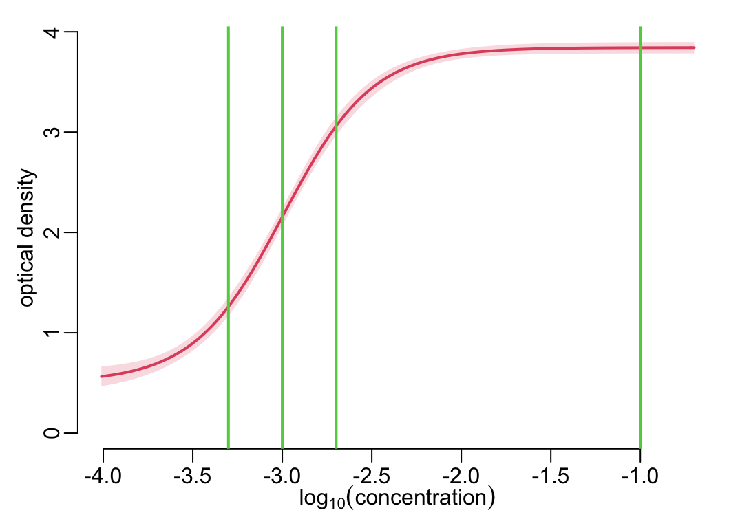
plot_standard_curve(standard_curve_df, anti_toxins); add_dilutions()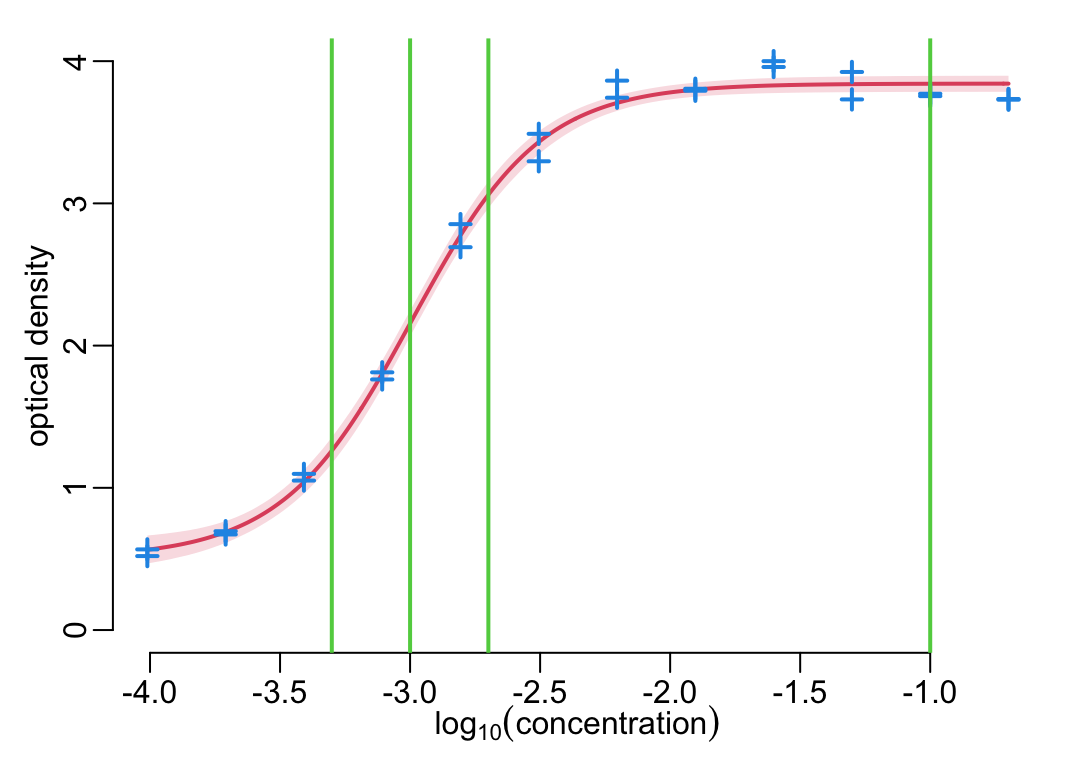
6 Processing all the plates
The four steps applied to all the plates (takes about 30”):
anti_toxins <- map(plates, get_antitoxins)
standard_curve_df <- map(anti_toxins, standard_curve_data, nls4PL)
standard_curves <- map(standard_curve_df, data2function)
samples <- map2(plates, standard_curves, process_samples)
6.1 The standard curves
Showing all the standard curves together:
xs <- map(standard_curve_df, ~ .x$logc)
ys <- map(standard_curve_df, ~ .x$median)
plot_frame(unlist(xs), unlist(ys))
walk2(xs, ys, lines2)
add_dilutions()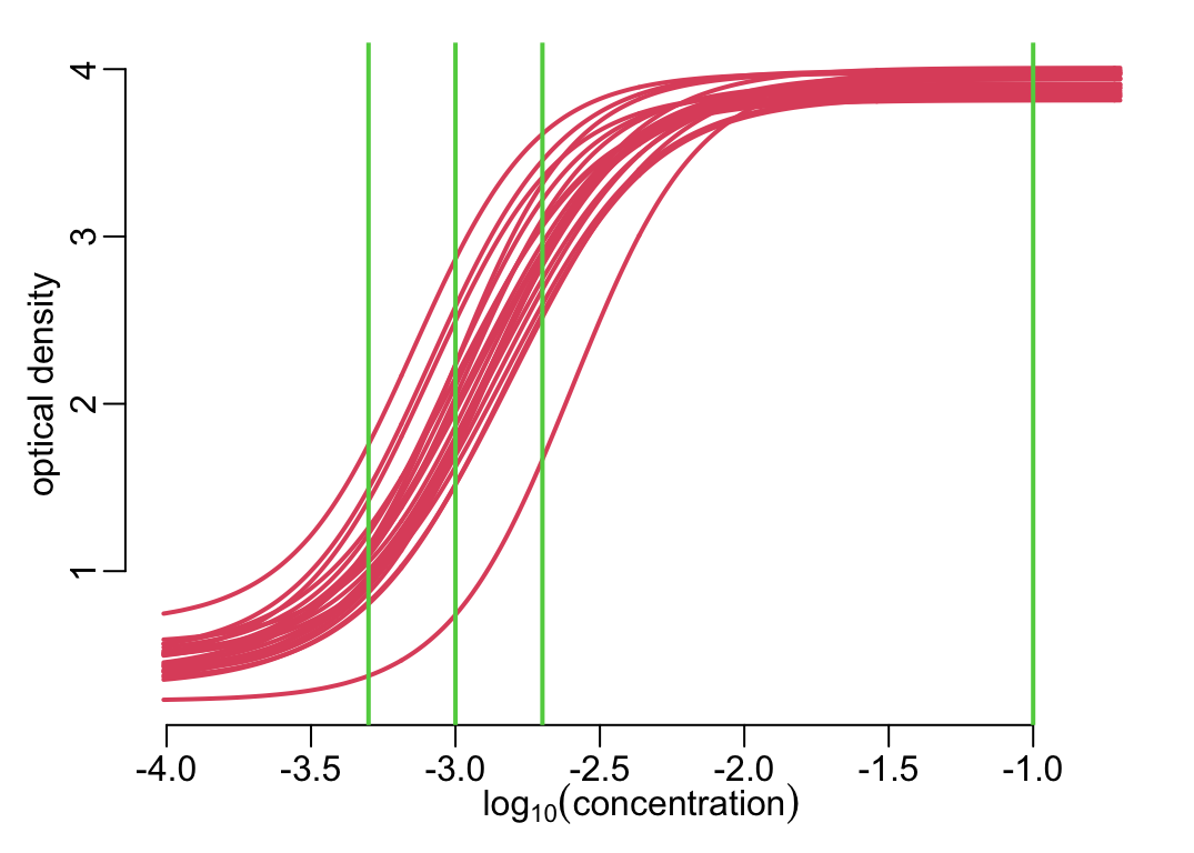
Showing the standard curves and data points, plate by plate:
titles <- anti_toxins |>
  names() |>
  str_remove("_hcdc") |>
  str_replace("_", " ")

opar <- par_mfrow(c(8, 3))
walk(seq_along(anti_toxins), function(i) {
  plot_standard_curve(standard_curve_df[[i]], anti_toxins[[i]], ylim = c(- .2, 4))
  mtext(titles[i], line = -4, at = -1.5)
})
par(opar)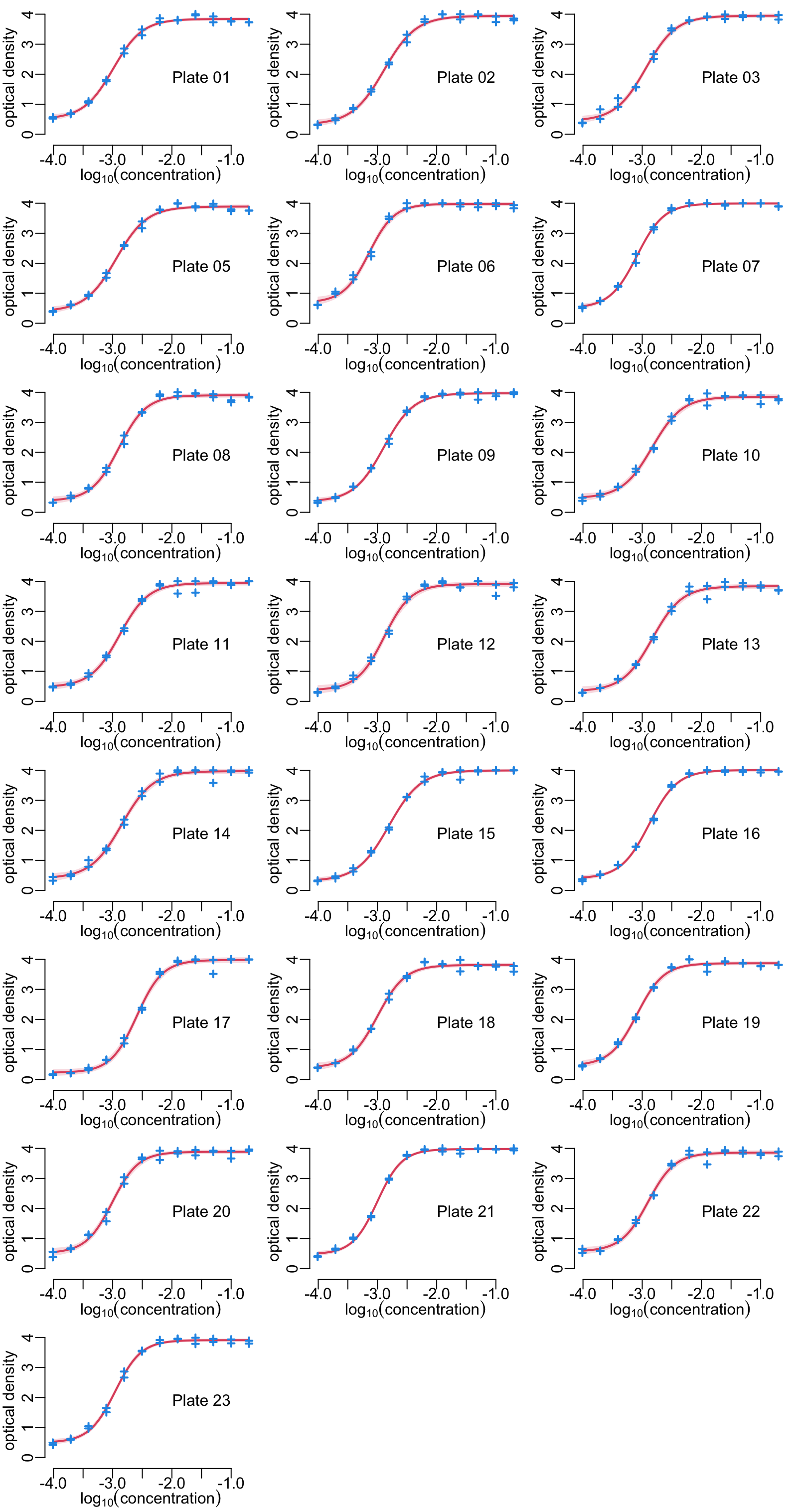
Showing the distributions of the ODs for the 3 dilutions, across the plates, together with the standard curves:
dilutions <- map_dfc(dilutions_factors,
    function(x) map(samples, ~ .x |>
                               filter(DILUTION_FACTORS == x) |>
                               pull(RESULT)) |> unlist())

xlim <- c(-.3, 4.1)
hist2 <- function(x, y, ...) {
  plot(unlist(ys), unlist(xs), type = "n", xaxs = "i", xlim = xlim,
     xlab = "optical density", ylab = bquote(log[10](concentration)))
  walk2(ys, xs, lines2)
  par(new = TRUE)
  hist(x, breaks = seq(0, 4, .1), col = color_data, xaxs = "i",
       axes = FALSE, ann = FALSE, xlim = xlim, ylim = c(0, 300), , ...)
  axis(4); mtext("number of samples", 4, 1.5)
  abline(v = c(.8, 3.8), lty = 2)
  mtext(y, 3, -1, font = 2)
}

opar <- par_mfrow(c(3, 1))
walk2(dilutions, paste("Dilution", dilutions_factors), hist2)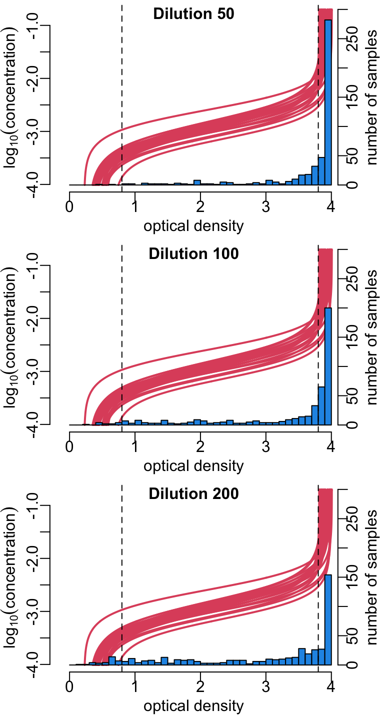
par(opar)6.2 Concentrations
Plotting the concentration estimates per plates and dilution for all the samples:
plot_concentrations <- function(x) {
  nb_replicates <- unique(table(x$HCDC_SAMPLE_ID))
  nb <- nrow(x)
  colors <- rep(2:4, nb / nb_replicates)
  tmp <- (1:(nb + nb / nb_replicates - 1))
  vertical_lines <- seq(nb_replicates + 1,
                        tail(tmp, nb_replicates + 1)[1],
                        nb_replicates + 1)
  xs <- tmp[-vertical_lines]
  x |>
    mutate(across(c(lower, median, upper), ~ 10^.x * DILUTION_FACTORS)) |>
    with({
      plot(xs, median, col = colors, lwd = lwd_val,
           ylim = c(0, max(median, upper, na.rm = TRUE)),
           axes = FALSE, xlab = NA, ylab = "concentration (IU/mL)")
      axis(2)
      segments(xs, lower, xs, upper, col = colors, lwd = lwd_val)
    })
  abline(v = vertical_lines, col = "grey")
  abline(h = .1, col = "grey")
}

opar <- par_mfrow(c(11, 2))
walk2(samples, titles, ~ {plot_concentrations(.x); mtext(.y)})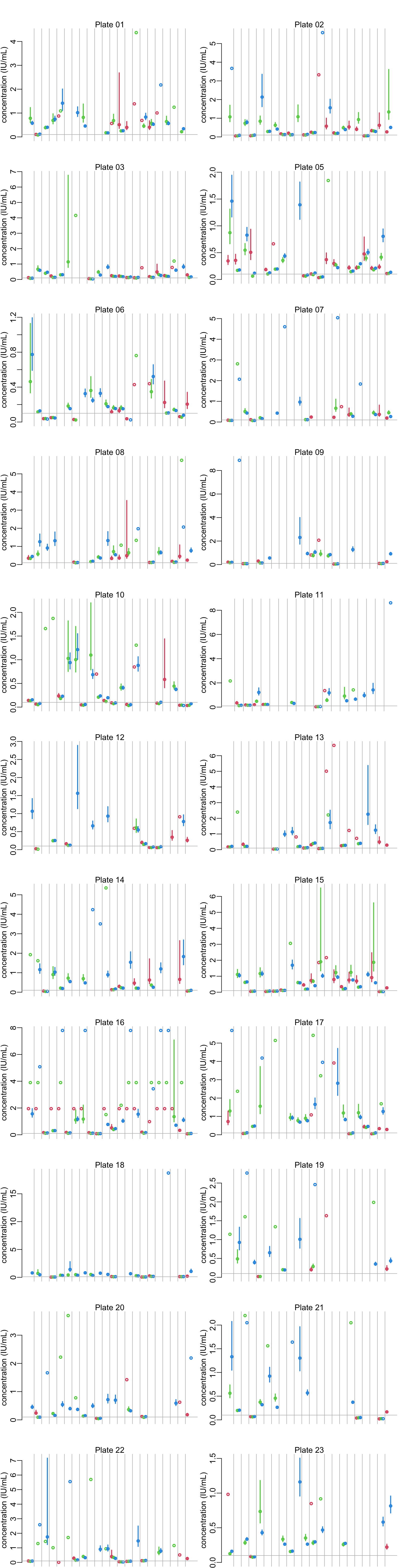
par(opar)6.3 Looking at the dilutions
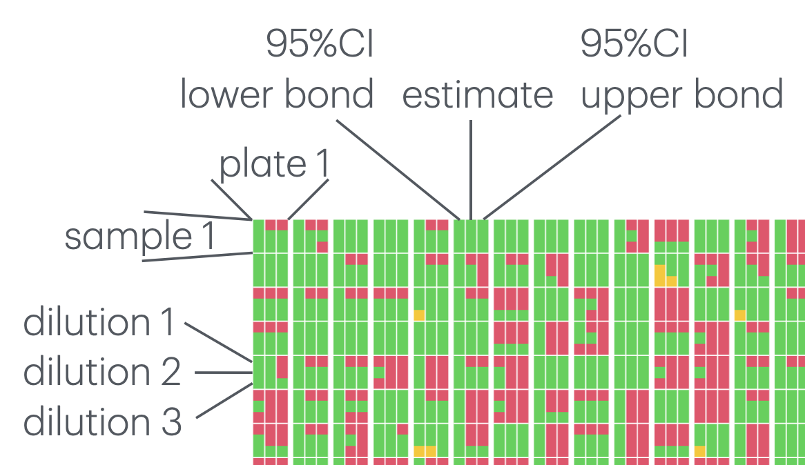
Showing where estimates are possible (in green). When they are not possible, it’s either because the concentration is too high (in red), or because the concentration is too low (in orange). Each of the 22 columns represents a plate and each of the 22 rows with each column represents a sample. Within each sample, the 3 columns are for the point estimates of the concentrations (middle) with 95% confidence interval (lower and upper bounds in the left and right columns respectively) and the 3 rows are for the 3 dilutions values (50, 100 and 200 from top to bottom):
# function to add missing values if there are less than 22 samples in a plate:
nb_smpls <- 22 # number of samples per plate
nb_dltns <- 3 # number of dilutions per sample
nb_estmts <- 3 # number of estimates per dilution (point + confidence interval)
template <- matrix(rep(NA, nb_smpls * nb_dltns * nb_estmts), nrow = nb_estmts)
format_mat <- function(x) {
  template[, 1:ncol(x)] <- x
  template
}

# the function that draws the heatmap for 1 plate:
abline2 <- function(...) abline(..., col = "white")
plot_heatmap <- function(x) {
  x |>
    mutate(across(c(lower, median, upper),
                  ~ as.numeric(is.na(.x)) * ((RESULT > 2) + 1))) |>
    select(lower, median, upper) |>
    as.matrix() |>
    t() |>
    format_mat() |>
    (\(.x) .x[, ncol(.x):1])() |>
    (\(.x) image(1:nb_estmts, 1:(nb_smpls * nb_dltns), .x,
                 axes = FALSE, ann = FALSE, col = c(3, 7, 2)))()

  abline2(v = c(1.5, 2.5))
  abline2(h = seq(nb_dltns, nb_dltns * nb_smpls, nb_dltns) + .5)
}

opar <- par(mfrow = c(1, 22))
walk(samples, plot_heatmap)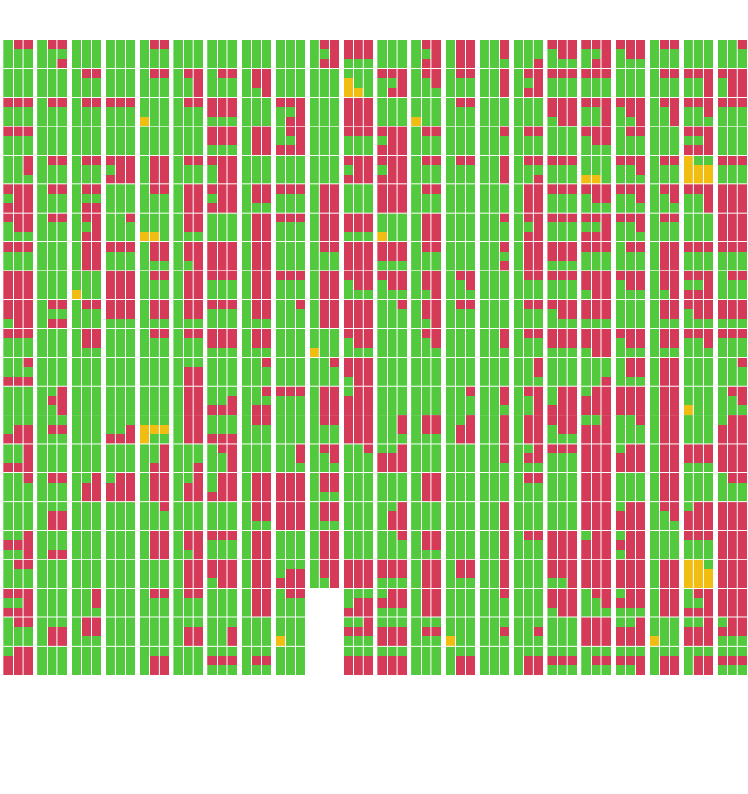
par(opar)This is how to interprete the above figure:
Number of samples for which a concentration can be estimated:
nb_NA <- samples |>
  bind_rows() |>
  mutate(total =  is.na(lower) + is.na(median) + is.na(upper))

# with full confidence interval:
nb_NA |>
  group_by(HCDC_SAMPLE_ID) |>
  summarise(OK = any(total < 1)) |>
  pull(OK) |>
  sum()
[1] 339# with partial confidence interval:
nb_NA |>
group_by(HCDC_SAMPLE_ID) |>
summarise(OK = any(total < 2)) |>
pull(OK) |>
sum()[1] 388Out of 481 samples,
- there are 2 sample (0.4 %) for which a dilution of 50 is already too much in order to estimate the lower bound of its 95% confidence interval;
- there are 340 samples (70.6 %) for which the concentration can be estimated with a 95% confidence interval.
- and an additional 47 samples (9.8 %) for which the concentration can be estimated with a partial 95% confidence interval.
Let’s look at the optimal dilution for each sample:
concentrations_estimates <- samples |>
  bind_rows() |>
  select(HCDC_SAMPLE_ID, DILUTION_FACTORS, RESULT, lower, median, upper) |>
  mutate(across(c(lower, median, upper), ~ DILUTION_FACTORS * 10^.x),
         ci_range   = upper - lower)

best_estimates <- concentrations_estimates |>
  group_by(HCDC_SAMPLE_ID) |>
  filter(ci_range == min(ci_range, na.rm = TRUE)) |>
  ungroup()

optimal_dilutions <- best_estimates |>
  pull(DILUTION_FACTORS) |>
  table()

optimal_dilutions
 50 100 200
80 78 181 round(100 * optimal_dilutions / 340, 1)
  50  100  200
23.5 22.9 53.2
Meaning that, out of the 340 samples for which an estimate with confidence interval can be generate, 80 (23.5%) have an optimal dilution of 50, 78 (22.9%) have an optimal dilution of 100 and 182 (53.5%) have an optimal dilution of 200.
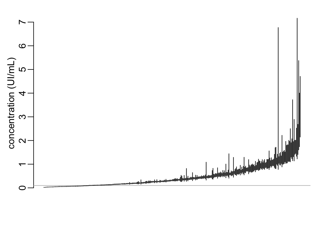
The estimates with the full confidence interval:
ticks <- 1:nrow(best_estimates)
with(best_estimates,
     plot(ticks, median, ylim = c(0, max(upper)), type = "n", axes = FALSE, xlab = NA,
          ylab = "concentration (UI/mL)"))
axis(2)
abline(h = .1, col = "grey")

best_estimates |>
  arrange(median, ci_range) |>
  with({
    segments(ticks, lower, ticks, upper)
  })
The number of missing estimates (point or any of tbe bounds of the confidence interval) as a function of the dilution:
# A function that adds axes and grid:
add_grid <- function() {
  axis(1); axis(2, 0:3)
  abline(h = 0:3, col = "grey")
  abline(v = c(50, 100, 200), col = "grey")
}

plot3 <- function(...) {
  plot2(..., axes = FALSE, xlab = "dilution", ylab = "number of missing estimates")
}

# Preparing the data:
nb_missing <- nb_NA |>
  group_by(DILUTION_FACTORS, total) |>
  tally() |>
  ungroup()

mean_nb_missing <- nb_missing |>
  group_by(DILUTION_FACTORS) |>
  mutate(mean = sum(total * n) / sum(n)) |>
  ungroup() |>
  select(- total,  - n) |>
  unique()

# The plot:
with(nb_NA, plot3(jitter(DILUTION_FACTORS), jitter(total)))
with(mean_nb_missing, lines(DILUTION_FACTORS, mean, lwd = 2, col = 2))
add_grid()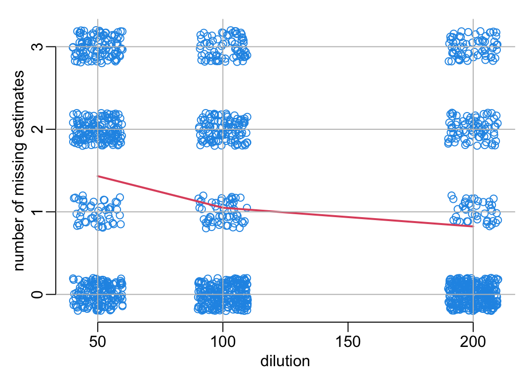
An alternative plot:
with(nb_missing, plot3(DILUTION_FACTORS, total, cex = sqrt(n) / sqrt(min(n)), pch = 19,
                       xlim = c(45, 205), ylim = c(-.2, 3.3)))
with(mean_nb_missing, lines(DILUTION_FACTORS, mean, lwd = 2, col = 2))
add_grid()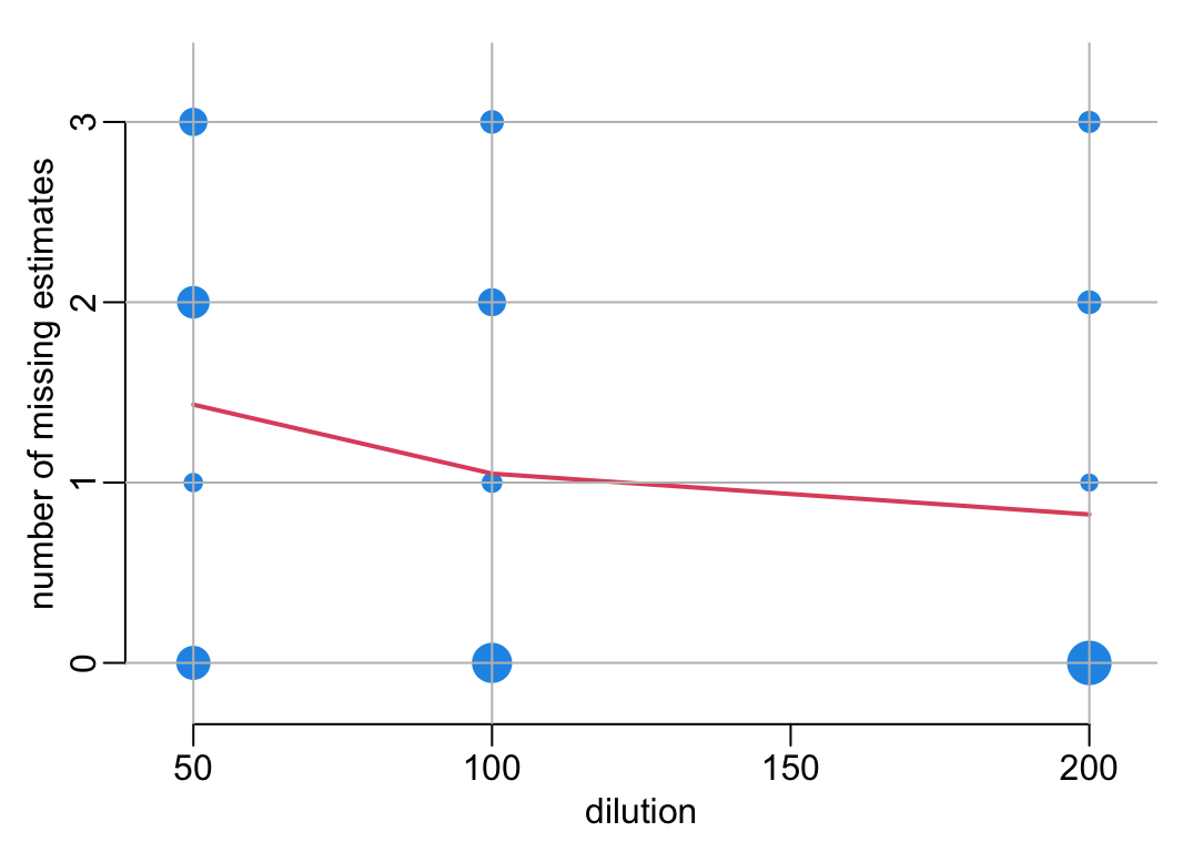
6.4 Exporting the estimates
best_estimates |>
  select(- ci_range) |>
  write_delim2("concentrations_estimates.csv")
7 Negative controls
A function that retrieves the negative controls from 1 plate:
get_negatives_controls <- function(x) {
  x |>
    select(starts_with("NEGATIVE")) |>
    unique() |>
    tidyr::pivot_longer(everything(), names_to = "dilution", values_to = "od") |>
    mutate(across(dilution, ~ stringr::str_remove(.x, "NEGATIVE_") |> as.integer()))
}
Retrieving all the negative controls of all the plates and computing the concentrations:
neg_contr <- plates |>
  map_dfr(get_negatives_controls, .id = "plate") |>
  rowwise() |>
  mutate(concentration = list(10^standard_curve(od))) |>
  tidyr::unnest_wider(concentration) |>
  mutate(across(c(lower, median, upper), ~ .x * dilution),
         ci_range = upper - lower,
         positive = ! upper < positive_threshold)
Selecting the best dilution for each sample and checking that the negative control are identified as negative:
neg_contr |>
  group_by(plate) |>
  filter(ci_range == min(ci_range, na.rm = TRUE)) |>
  ungroup() |>
  print_all()
# A tibble: 22 × 8
plate dilution od lower median upper ci_range positive
<chr> <int> <dbl> <dbl> <dbl> <dbl> <dbl> <lgl>
1 Plate_01_hcdc 50 1.74 0.0347 0.0372 0.0399 0.00526 FALSE
2 Plate_02_hcdc 50 1.45 0.0274 0.0298 0.0322 0.00485 FALSE
3 Plate_03_hcdc 50 2.39 0.0553 0.0588 0.0626 0.00734 FALSE
4 Plate_05_hcdc 50 1.84 0.0376 0.0402 0.0431 0.00541 FALSE
5 Plate_06_hcdc 50 1.72 0.0343 0.0369 0.0395 0.00524 FALSE
6 Plate_07_hcdc 100 1.24 0.0445 0.0490 0.0535 0.00900 FALSE
7 Plate_08_hcdc 50 1.27 0.0230 0.0252 0.0275 0.00453 FALSE
8 Plate_09_hcdc 50 1.69 0.0334 0.0359 0.0386 0.00519 FALSE
9 Plate_10_hcdc 50 1.58 0.0305 0.0329 0.0355 0.00501 FALSE
10 Plate_11_hcdc 50 1.26 0.0227 0.0249 0.0272 0.00452 FALSE
11 Plate_12_hcdc 50 0.837 0.0121 0.0142 0.0162 0.00413 FALSE
12 Plate_13_hcdc 50 0.866 0.0129 0.0150 0.0170 0.00410 FALSE
13 Plate_14_hcdc 50 1.33 0.0244 0.0268 0.0291 0.00466 FALSE
14 Plate_15_hcdc 50 0.826 0.0117 0.0139 0.0159 0.00416 FALSE
15 Plate_16_hcdc 50 0.961 0.0155 0.0175 0.0196 0.00410 FALSE
16 Plate_17_hcdc 50 1.04 0.0175 0.0195 0.0217 0.00419 FALSE
17 Plate_18_hcdc 50 1.62 0.0316 0.0341 0.0367 0.00507 FALSE
18 Plate_19_hcdc 50 1.83 0.0373 0.0398 0.0426 0.00538 FALSE
19 Plate_20_hcdc 50 1.36 0.0252 0.0275 0.0299 0.00472 FALSE
20 Plate_21_hcdc 50 1.46 0.0275 0.0299 0.0324 0.00486 FALSE
21 Plate_22_hcdc 50 0.847 0.0124 0.0145 0.0165 0.00411 FALSE
22 Plate_23_hcdc 50 1.03 0.0172 0.0193 0.0214 0.00417 FALSE 8 New dilutions
Loading the data:
test <- readxl::read_excel(paste0(path2data,
                                  "Tetanus_Mr. Thanh FORMAT_TESTING STAFF.xlsx")) |>
  mutate(od = RESULT)
Calibrating the standard curve:
anti_toxins_test <- get_antitoxins(test)
standard_curve_df_test <- standard_curve_data(anti_toxins_test, nls4PL)
standard_curve_test <- data2function(standard_curve_df_test)
samples_test <- process_samples(test, standard_curve_test)
plot_standard_curve(standard_curve_df_test, anti_toxins_test)
add_dilutions()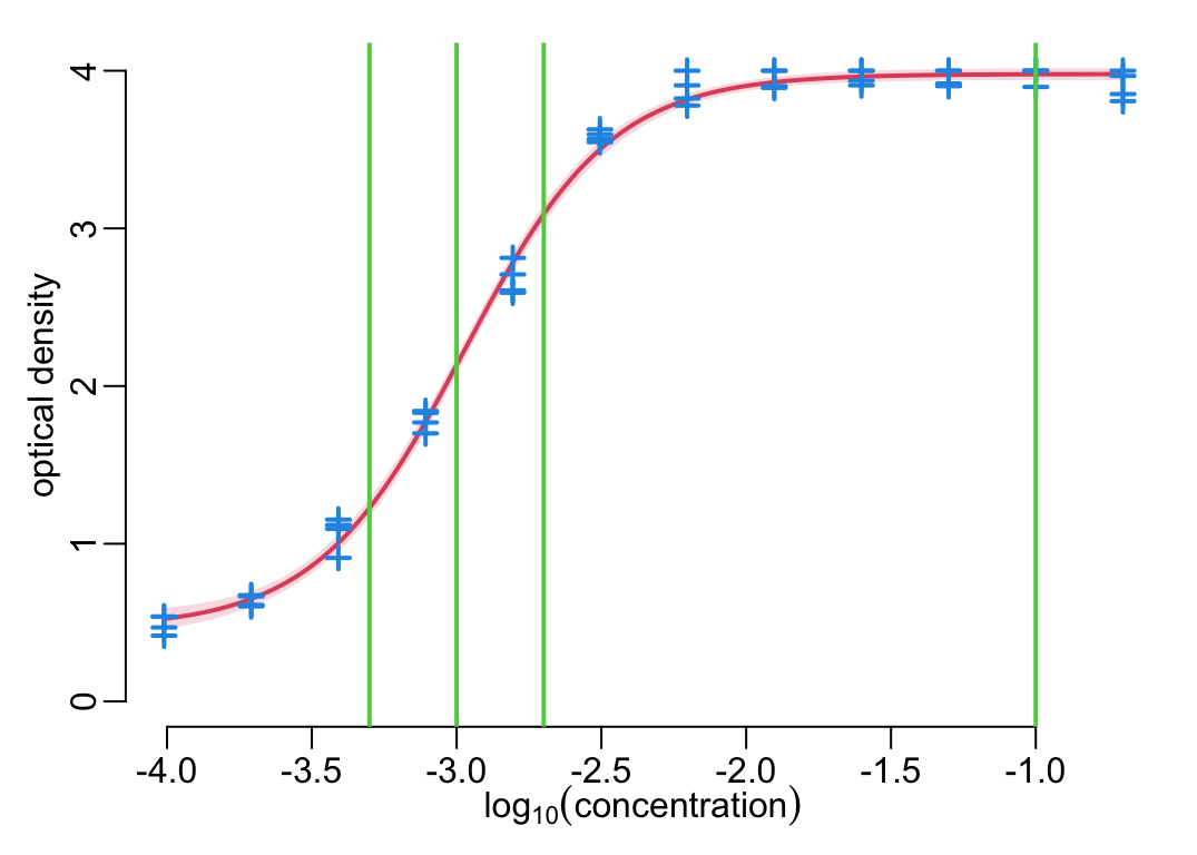
Estimating samples concentrations:
samples_test |>
  select(HCDC_SAMPLE_ID, DILUTION_FACTORS, RESULT, lower, median, upper) |>
  mutate(across(c(lower, median, upper), ~ DILUTION_FACTORS * 10^.x),
         ci_range   = upper - lower) |>
  group_by(HCDC_SAMPLE_ID) |>
  filter(ci_range == min(ci_range, na.rm = TRUE)) |>
  ungroup() |>
  select(- ci_range)
# A tibble: 4 × 6
HCDC_SAMPLE_ID DILUTION_FACTORS RESULT lower median upper
<chr> <dbl> <dbl> <dbl> <dbl> <dbl>
1 S1_A 400 3.16 0.811 0.856 0.907
2 S2_H 200 3.89 1.49 1.81 2.37
3 S5_TR 100 1.47 0.0588 0.0620 0.0651
4 S6_NC 50 3.68 0.194 0.212 0.235 9 Luminex data
9.1 First assay
Loading the data:
luminex <- readxl::read_excel(paste0(path2data,
                                     "Tetanus Luminex raw data-test01042025.xlsx")) |>
  rename(od = `Mean Fluorescence Intensity (MFI)`,
         HCDC_SAMPLE_ID = Sample)
The dilutions are the following:
sort(unique(luminex$DILUTION_FACTORS)) [1] 25 50 100 200 400 800 1600 3200 6400 12800
[11] 25600 51200 102400Plotting the anti-toxin data:
xlim <- c(-4.4, -.75)
col_elisa <- 2
col_luminex <- 4

anti_toxins_luminex <- get_antitoxins(luminex)
plot(unlist(xs), unlist(ys), xlim = xlim, axes = FALSE, ylab = NA, type = "n",
     xlab = bquote(log[10](concentration)))
axis(1)
axis(2, col = col_elisa, col.axis = col_elisa)
mtext("optical density", 2, line = 1.5, col = col_elisa)
walk2(xs, ys, lines2)

par(new = TRUE)
with(anti_toxins_luminex,
     plot2(log10(concentration), od, ylab = "MFI", xlim = xlim, lwd = lwd_val,
           axes = FALSE, ann = FALSE))
anti_toxins_luminex |>
  group_by(concentration) |>
  summarize(od = mean(od)) |>
  with(lines(log10(concentration), od, lwd = lwd_val, col = color_data))
axis(2, line = -3, col = col_luminex, col.axis = col_luminex)
mtext("median fluorescence intensity", 2, line = -1.5, col = col_luminex)

add_dilutions();
abline(v = log10(positive_threshold / 25), col = "grey", lwd = lwd_val)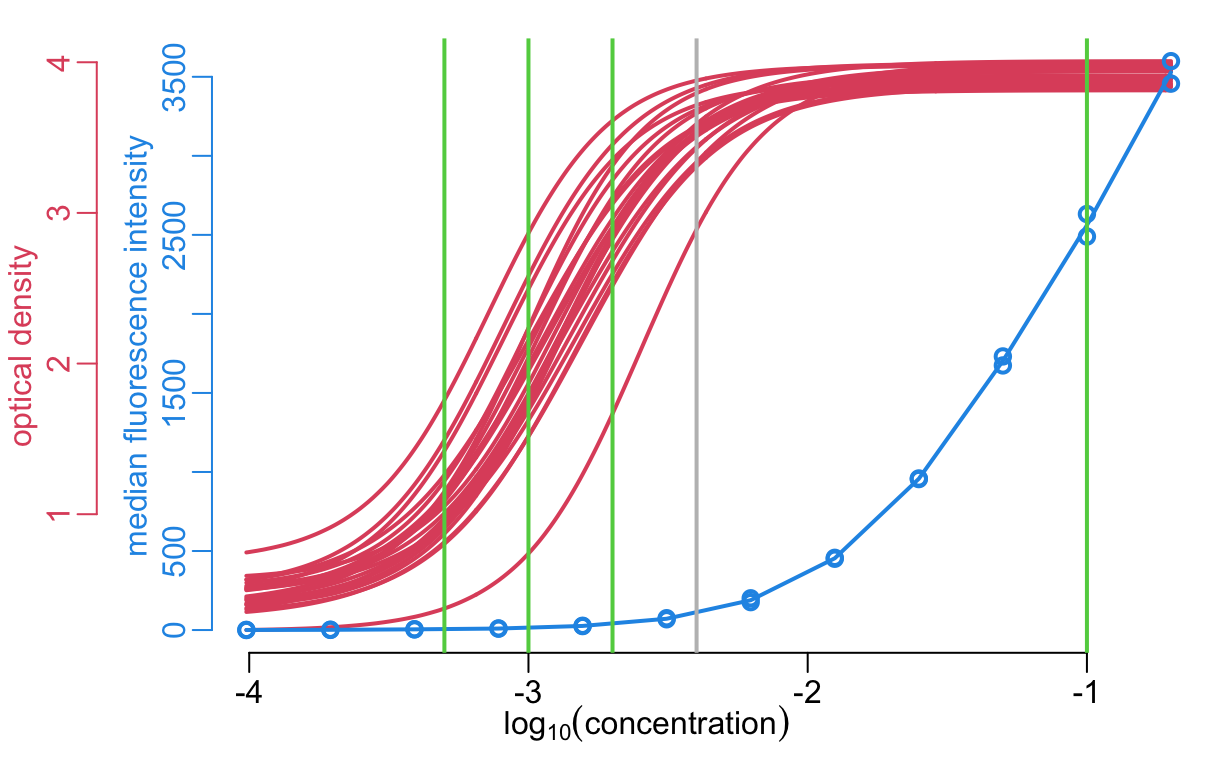
9.2 Second assay
Selection of samples:
high_concentrations <- samples |>
  bind_rows() |>
  arrange(desc(lower)) |>
  pull(HCDC_SAMPLE_ID) |>
  unique() |>
  head(10)

low_concentrations <- samples |>
  bind_rows() |>
  arrange(upper) |>
  pull(HCDC_SAMPLE_ID) |>
  unique() |>
  head(10)
A selection of high concentration samples:
high_concentrations [1] "U07B532207549" "U07B532300113" "U07B532207215" "U07B522205091"
[5] "U07B532207216" "U07B532207218" "U07B532207220" "U07B532207222"
[9] "U07B532207223" "U07B532207226"A selection of low concentration samples:
low_concentrations [1] "U07B522205309" "U07B522205149" "U07B532300109" "U07B522205067"
[5] "U07B522205077" "U07B522205288" "U07B522205063" "U07B532207252"
[9] "U07B522205188" "U07B522205294"Results:
luminex2 <- readxl::read_excel(paste0(path2data,
"Result for Marc_Tetanus Luminex raw data-& 20 samples july2025.xlsx"),
skip = 1, .name_repair = "unique_quiet") |>
rename(od = `Mean Fluorescence Intensity (MFI)`,
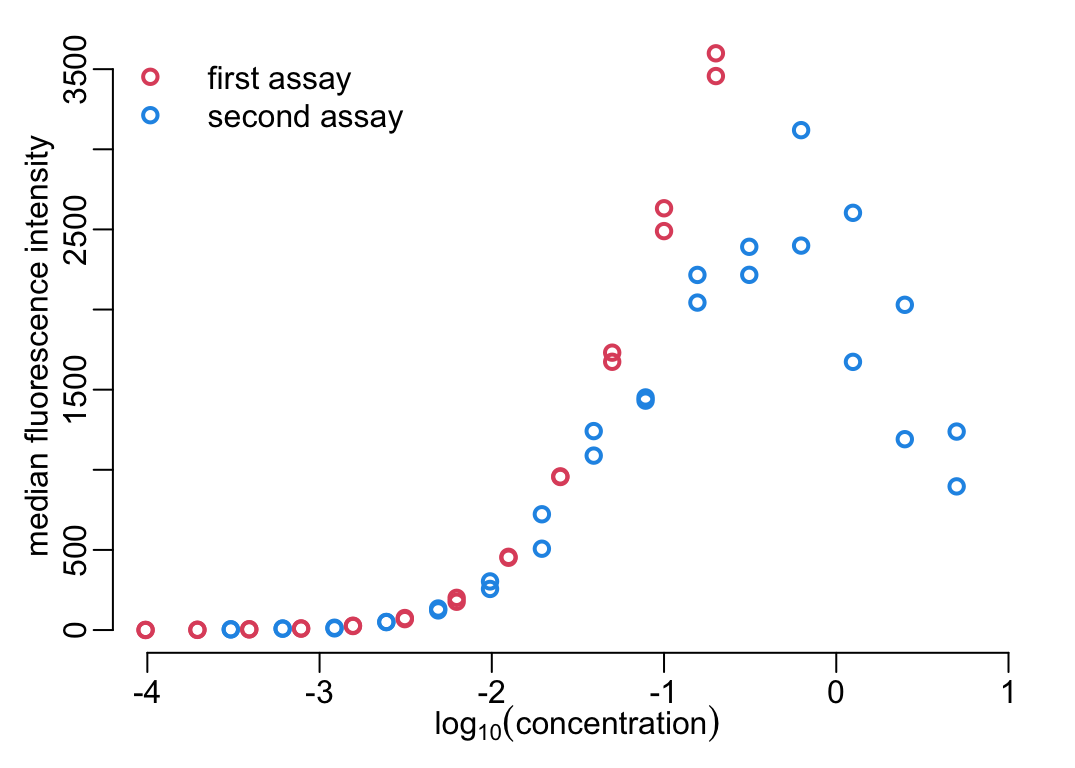
HCDC_SAMPLE_ID = Sample)Comparison with first assay:
anti_toxins_luminex2 <- get_antitoxins(luminex2)

with(anti_toxins_luminex2,
     plot2(log10(concentration), od, lwd = lwd_val,
           xlim = c(-4, 1), ylim = c(0, 3550),
           xlab = bquote(log[10](concentration)),
           ylab = "median fluorescence intensity"))

with(anti_toxins_luminex,
     points(log10(concentration), od, ylab = "MFI", lwd = lwd_val, col = 2))

legend("topleft", legend = c("first assay", "second assay"), pch = 1, lwd = lwd_val,
       col = c(2, 4), bty = "n", lty = 0)