library(purrr)
library(dplyr)Outbreaks simulations
Implementation of the method described in Noufaily et al. (2013).
Required packages:
A tuning of the dplyr::bind_col() function:
bind_cols2 <- function(...) dplyr::bind_cols(..., .name_repair = "unique_quiet")A tuning of the rpois() function:
rpois2 <- function(lambda) rpois(length(lambda), lambda)A tuning of the plot() function:
plot2 <- function(...) plot(..., type = "s", xlab = "week", ylab = "count")A function that generates the mean of the incidence as a function of time (in weeks) with trend and seasonality:
mu <- function(t, theta, beta, gamma1, gamma2, m) {
  t2 <- 2 * pi * t((1:m) %*% t(t)) / 52
  exp(theta + beta * t + rowSums(gamma1 * cos(t2) + gamma2 * sin(t2)))
}
A function that stochastically generates incidence as a function of time using the mean as generated by the above mu() function and a negative binomial distribution. This is how it should be done if the dispersion parameter \(\phi\) is interpreted correctly:
baseline1 <- function(n, t, theta, beta, gamma1, gamma2, phi, m) {
  counts <- mu(t, theta, beta, gamma1, gamma2, m)
  1:n |>
    map(~ rnbinom(t, phi, mu = counts)) |>
    bind_cols2()
}
This is how it’s done in the article:
baseline2 <- function(n, t, theta, beta, gamma1, gamma2, phi, m) {
  counts <- mu(t, theta, beta, gamma1, gamma2, m)
  prob <- 1 / phi
  size <- counts * prob / (1 - prob)
  1:n |>
    map(~ rnbinom(t, size, prob)) |>
    bind_cols2()
}
A function that generates the standard deviation of the incidence as a function of time, as it should be done if the dispersion parameter \(\phi\) is interpreted correctly:
stddev1 <- function(t, theta, beta, gamma1, gamma2, phi, m) {
  counts <- mu(t, theta, beta, gamma1, gamma2, m)
  sqrt(counts * (1 + counts / phi))
}
As it’s done in the article:
stddev2 <- function(t, theta, beta, gamma1, gamma2, phi, m) {
  sqrt(mu(t, theta, beta, gamma1, gamma2, m) * phi)
}
A function that simulates outbreak cases to add to non-outbreak cases:
outbreaks_cases <- function(stimes, stddev, indexes, k, weights) {
  k * stddev[stimes] |>
    rpois2() |>
    map2(stimes - 1, ~ c(rep(0, .y), round(.x * weights))[indexes]) |>
    bind_cols2() |>
    rowSums()
}
where stimes is a vector of outbreak starting times, stddev is a vector of the standard deviation of incidence as a function of time, indexes is a vector of indexes of the input time series (basically seq_along(stddev) here), k is the constant used for the rate of the Poisson distribution that determines the size of the outbreak, and weights is a vector of temporal weights used to spread the total number of cases during the outbreak along time. A function that adds outbreak cases to non-outbreak cases, using the above outbreaks_cases() function:
add_outbreak_cases <- function(weeks, stddev, nb, k, weights) {
  indexes <- seq_along(stddev)
  1:ncol(weeks) |>
    map(~ sample(indexes, nb)) |>
    bind_cols2() |>
    map(outbreaks_cases, stddev, indexes, k, weights) |>
    bind_cols2() |>
    magrittr::add(weeks)
}
where weeks is the time series of non-outbreak cases and nb is the number of outbreaks we wish to add to the time series of incidence. The simulator that puts together all the above functions:
simulator <- function(n = 12 * 52, N = 100,
                      theta = 1.5, beta = .003, gamma1 = .2, gamma2 = -.4,
                      phi = 1, m = 1,
                      baseline_function = baseline1,
                      stddev_function = stddev1,
                      baseline_from = 313, baseline_to = 575,
                      current_from = 576, current_to = NULL,
                      meanlog = 0, sdlog = .5,
                      nb_outbreaks_baseline = 4, nb_outbreaks_current = 1, k = 2) {

  if (is.null(current_to)) current_to <- n
  baseline_indexes <- baseline_from:baseline_to
  current_indexes <- current_from:current_to

  t_vals <- 1:n
  t_weights <- diff(c(0, plnorm(seq_along(t_vals), meanlog, sdlog)))

  baseline_vals <- baseline_function(N, t_vals, theta, beta, gamma1, gamma2, phi, m)
  stddev_vals <- stddev_function(t_vals, theta, beta, gamma1, gamma2, phi, m)

  baseline_weeks <- baseline_vals[baseline_indexes, ]
  baseline_stddev <- stddev_vals[baseline_indexes]

  current_weeks <- baseline_vals[current_indexes, ]
  current_stddev <- stddev_vals[current_indexes]

  list(bsln_outbrk = add_outbreak_cases(baseline_weeks, baseline_stddev,
                                        nb_outbreaks_baseline, k, t_weights),
       curr_outbrk = add_outbreak_cases(current_weeks, current_stddev,
                                        nb_outbreaks_current, k, t_weights))
}
The scenarios of Figure 2:
scenarios <- list(
  s8  = list(theta = - 2,   beta = 0,     gamma1 =  .1, gamma2 =   .3, phi = 2, m = 1),
  s10 = list(theta = - 2,   beta =  .005, gamma1 = 0,   gamma2 =  0,   phi = 2, m = 0),
  s12 = list(theta = - 2,   beta =  .005, gamma1 =  .1, gamma2 =   .3, phi = 2, m = 2),
  s17 = list(theta =   1.5, beta =  .003, gamma1 =  .2, gamma2 = - .4, phi = 1, m = 1))
Generating the data for Figure 2:
set.seed(30101976)
t_vals <- 1:(12 * 52)

data_fig2_1 <- scenarios |>
  map(~ with(.x, baseline1(n = 1, t = t_vals, theta = theta, beta = beta,
                           gamma1 = gamma1, gamma2 = gamma2, phi = phi, m = m))) |>
  map(unlist)

data_fig2_2 <- scenarios |>
  map(~ with(.x, baseline2(n = 1, t = t_vals, theta = theta, beta = beta,
                           gamma1 = gamma1, gamma2 = gamma2, phi = phi, m = m))) |>
  map(unlist)
Figure 2 as it should be done:
opar <- par(mfrow = c(2, 2), plt = c(.12, 1, .18, .98))
walk(data_fig2_1, ~ plot2(t_vals, .x))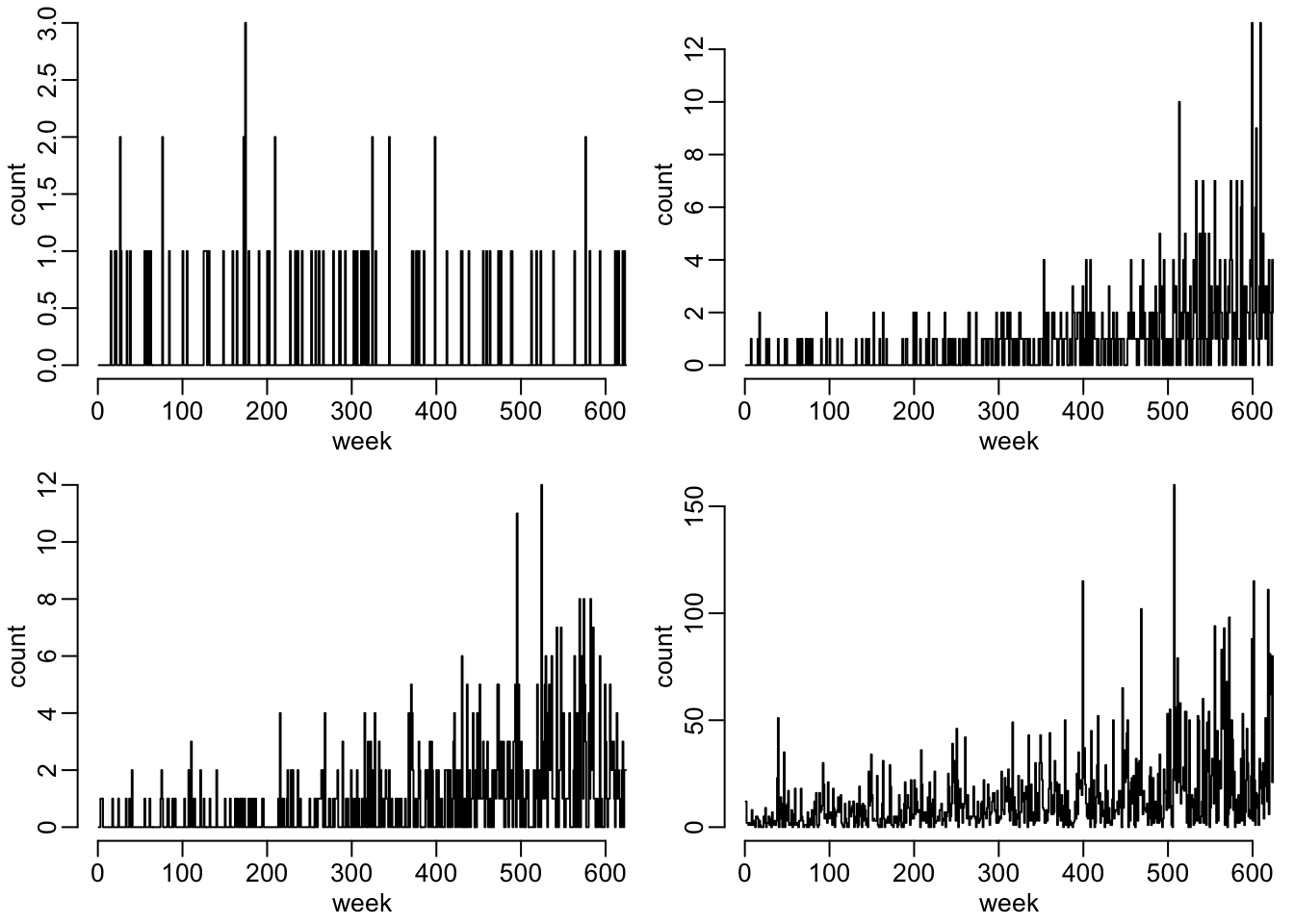
par(opar)Figure 2 as it’s done in the article:
opar <- par(mfrow = c(2, 2), plt = c(.12, 1, .18, .98))
walk(data_fig2_2, ~ plot2(t_vals, .x))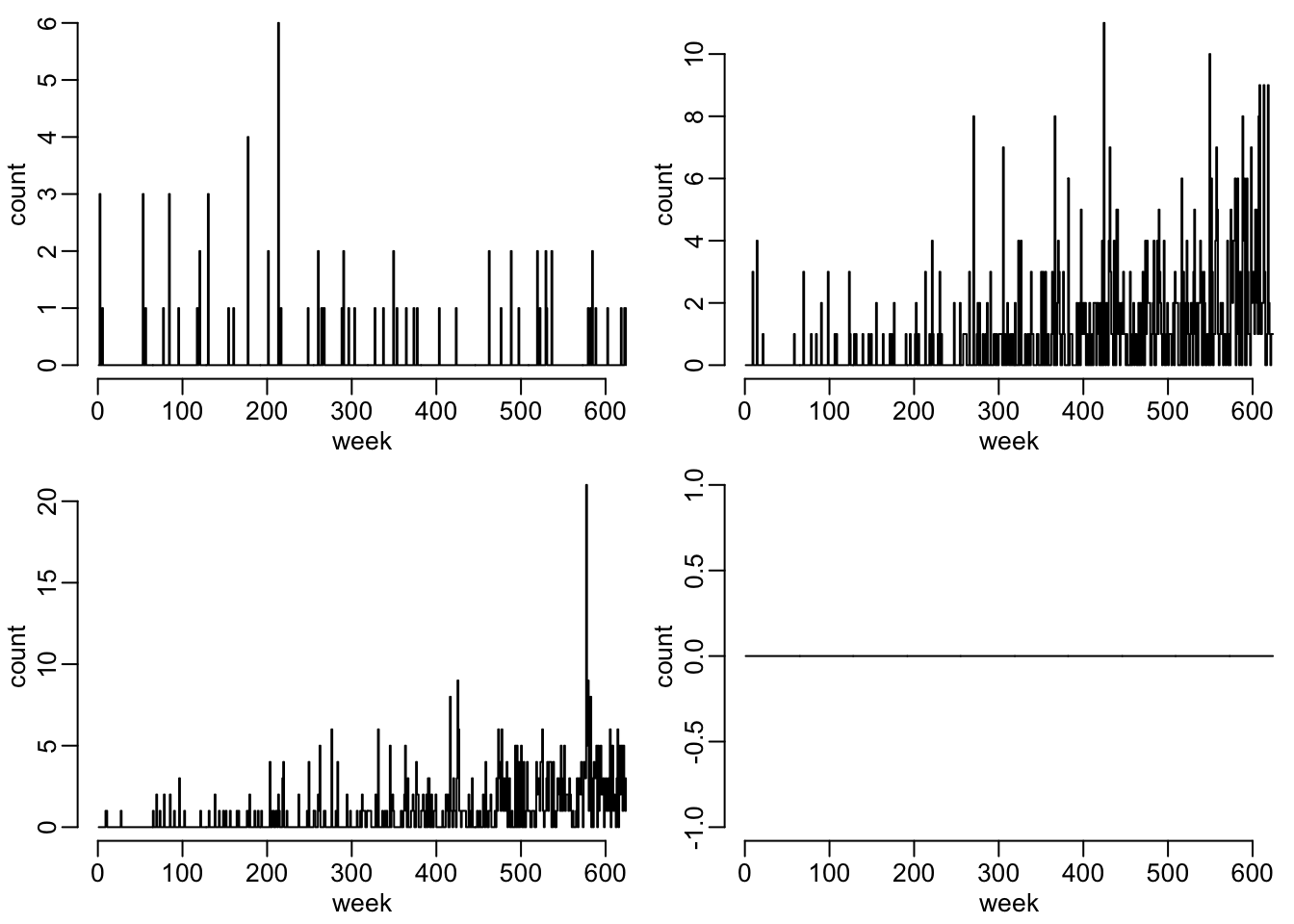
par(opar)There seems to be something wrong with scenario 17… Let’s now run the simulator with the outbreaks for the 4 scenarios and the 2 options regarding the dispersion parameter:
simulations1 <- map(scenarios,
                    ~ with(.x, simulator(theta = theta, beta = beta, gamma1 = gamma1,
                                         gamma2 = gamma2, phi = phi, m = m,
                                         baseline_function = baseline1,
                                         stddev_function = stddev1)))

simulations2 <- map(scenarios,
                    ~ with(.x, simulator(theta = theta, beta = beta, gamma1 = gamma1,
                                         gamma2 = gamma2, phi = phi, m = m,
                                         baseline_function = baseline2,
                                         stddev_function = stddev2)))
Values considered for \(k\) is the article: 2, 3, 5 and 10.
References
Noufaily, A., D. G. Enki, P. Farrington, P. Garthwaite, N. Andrews, and A. Charlett. 2013. An improved algorithm for outbreak detection in multiple surveillance systems. Statistics in Medicine 32:1206–1222.