path2data <- paste0(Sys.getenv("HOME"), "/Library/CloudStorage/",
                    "OneDrive-OxfordUniversityClinicalResearchUnit/",
"GitHub/choisy/60HN/")60HN: CRE burden at admission and discharge
The all code takes about 10’ to run in parallel.
1 Constants
The folder that contains the data files:
The name of the file that contains the discharge dates of the patients that did not provide samples at discharge:
discharge_file <- "60HN - DischargeDate_no_discharge_sample_27Nov25.xlsx"The name of the CRF data file:
CRF_file <- "16-12-2025-_60HN_PATIENT_P1_Data.xls"The name of the MALDI-TOF data file:
MALDITOF_file <- "60HN_ID_MALDITOF_confirmation_20251128.xlsx"Number of minutes per day:
mpd <- 1440The number of cores to use for parallel computing:
nb_cores <- parallel::detectCores() - 1
#nb_cores <- 1
2 Packages
Required packages:
required <- c("readxl", "purrr", "dplyr", "lubridate", "magrittr", "tidyr", "msm",
              "rlang", "mgcv", "gratia", "alluvial", "furrr")
Installing those that are not installed yet:
to_install <- required[! required %in% installed.packages()[,"Package"]]
if (length(to_install)) install.packages(to_install)
Loading the packages for interactive use:
invisible(sapply(required, library, character.only = TRUE))Setting the strategy of the furrr package:
plan(multisession)3 General functions
A tuning of the readRDS() function:
readRDS2 <- function(x) readRDS(paste0(path2data, x))A function that pastes a vector of dates and a vector of times both in character format and returns a dttm vector:
as_datetime2 <- function(date, time) {
  as_datetime2_ <- function(date, time) {
    if (is.na(date)) return(NA)
    if (is.na(time)) time <- "12:00:00"    # if only time is missing, we fix it to noon
    as_datetime(paste(date, time))
  }
  map2_vec(date, time, as_datetime2_)
}
A function that converts a column col of a data frame x into a list-column (assuming that all the other columns have the same values across rows):
col2listcol <- function(x, col) {
  x |>
    select(- {{ col }}) |>
    first() |>
    bind_cols(tibble("{{col}}" := list(pull(x, {{ col }}))))
}
A tuning of the hist() function:
hist2 <- function(x, ...) hist(x, floor(min(x)):ceiling(max(x)), main = NA, ...)A wrapper that formats the output of the binom.test() function:
binom_test <- function(x, n, ...) {
  if (n < 1) return(c(estimate = NA, lower = NA, upper = NA))
  binom.test(x, n, ...) |>
    magrittr::extract(c("estimate", "conf.int")) |>
    unlist() |>
    setNames(c("estimate", "lower", "upper"))
}
A tuning of the polygon() function:
polygon2 <- function(x, y1, y2, border = NA, ...) {
  polygon(c(x, rev(x)), c(y1, rev(y2)), border = border, ...)
}
Utility functions to convert coordinates to make a stairs plot style:
x_transform <- function(x) c(x[1], rep(x[-1], each = 2))
y_transform <- function(y) c(rep(head(y, -1), each = 2), last(y))
A function that returns the indexes of the first values of consecutive NAs of a vector:
firstNA <- function(x) {
  y <- which(is.na(x))
  z <- diff(y) == 1
  if (any(z)) return(y[-(which(z) + 1)])
  y
}
Example use:
firstNA(c(1, 3, 2, 5, 3, NA, NA, 3, 2, 5, NA, 5, 3, 2, 6, NA, NA, NA, 1, 3, 2, 5, 3))[1] 6 11 16A function that duplicates the first rows of a series of rows with NA values in the colNA column, and replaces the values of the col_sel columns with values of the row right before:
duplicate_NA_rows <- function(x, colNA = "estimate",
                              col_sel = c("denominator", "numerator", "estimate",
                                          "lower", "upper")) {
  x <- mutate(x, .id = row_number())
  NA_ind <- firstNA(x[[colNA]])
  duplicates <- x[NA_ind, ]
  duplicates[, col_sel] <- x[NA_ind - 1, col_sel]
  duplicates |>
    bind_rows(x) |>
    arrange(.id) |>
    select(-.id)
}
A function that splits a data frame x into a list of data frames according to the presence of missing values in the col column of the data frame:
remove_NAs <- function(x, col) {
  x |>
    mutate(col1 = as.numeric(is.na({{ col }})),
           col2 = cumsum(col1)) |>
    na.exclude() |>
    group_by(col2) |>
    group_split()
}
Example use:
carbs <- mtcars$carb
carbs[c(8, 20:25)] <- NA
mtcars$carb <- carbs
remove_NAs(mtcars, carb)
rm(mtcars)
A tuning of the msm() function for a bi-state bi-directional case:
bsm <- function(formula, subject, data, ...) {
  output <- do.call(msm::msm, c(list(formula = formula,
                                     subject = substitute(subject),
                                     data    = data,
                                     qmatrix = matrix(c(0:1, 1:0), 2)), list(...)))
  output$call <- match.call()
  output
}
A function that bootstraps estimates of the fitted multistate model msm_fit where f is the function that generates the estimates and N is the number of bootstrap repetitions:
boot_msm <- function(msm_fit, f = qmatrix.msm, N = 1000, ...) {
  msm_fit |>
    boot.msm(function(x) f(x)$estimates, N, ...) |>
    unlist() |>
    array(dim = c(dim(msm_fit$Qmatrices$baseline), N))
}
A function that generates statistic f estimates from bootstrap samples boot_samples outputed by boot_msm():
boot_stat <- function(boots_samples, f = sd) {
  output <- apply(boots_samples, 1:2, f)
  mat_names <- paste("State", 1:nrow(output))
  colnames(output) <-  mat_names
  rownames(output) <-  mat_names
  output
}
A function that generates a ci% confidence interval from bootstrap samples boot_samples outputed by boot_msm():
boot_ci <- function(boots_samples, ci = .95) {
  ci <- (1 - ci) / 2
  output <- apply(boots_samples, 1:2, function(x) quantile(x, c(ci, 1 - ci)))
  mat_names <- paste("State", 1:ncol(output))
  dimnames(output) <- list(rownames(output[, , 1]), mat_names, mat_names)
  aperm(output, c(1, 3, 2))
}
A function that computes lubridate-formatted durations:
time_diff <- function(x) as.duration(diff(x))A function that extracts the estimations with 95% CI of the rate of colonization and decolonization per 100 patient days:
bsm_estimations <- function(x, event_names = c("colonization", "clearance")) {
  out <- cbind(matrix(x$estimates.t, 2), x$ci)
  rownames(out) <- event_names
  colnames(out) <- c("estimate", "lower", "upper")
  100 * out
}
Tunings of the alluvial() function:
alluvial2 <- alluvial
b <- body(alluvial2)
b[26] <- NULL
body(alluvial2) <- b

alluvial3 <- function(x, print = TRUE, ...) {
  alluvial2(x[, 1:2], freq = x[[3]], ...)
  if (print) return(x)
}
The following function returns the hazard ratio of the covariates (with 95% confidence intervals) of an output of msm():
HR <- function(x) summary(x)$hazard4 New data
PT_merged_not_identify_PSpatient <- readRDS2("PT_merged_not_identify_PSpatient.rds")
DT_merged_not_identify_PSpatient <- readRDS2("DT_merged_not_identify_PSpatient.rds")
5 Discharge dates
Loading the discharge dates for the patients who did not provide any sample at discharge:
(discharge_dates <- paste0(path2data, discharge_file) |>
  read_excel() |>
  mutate(across(`Discharge date`, ~ .x + hours(12))) |>  # setting time to noon
  select(-No, -SiteID, -`Discharge date (2)`))
# A tibble: 96 × 2
USUBJID `Discharge date`
<chr> <dttm>
1 010-3-1-05 2025-02-23 12:00:00
2 010-1-1-10 2025-02-24 12:00:00
3 010-1-1-22 2025-02-25 12:00:00
4 010-1-1-26 2025-02-28 12:00:00
5 010-2-1-09 2025-03-06 12:00:00
6 010-2-1-22 2025-03-06 12:00:00
7 010-3-1-09 2025-03-06 12:00:00
8 010-3-1-39 2025-03-23 12:00:00
9 010-3-1-36 2025-03-17 12:00:00
10 010-3-1-42 2025-03-25 12:00:00
# ℹ 86 more rows6 CRF data
Reading the data (it takes 1”):
file <- paste0(path2data, CRF_file)

CRF <- file |>
  excel_sheets() |>
  head(-1) |>
  set_names() |>
  map(read_excel, path = file) |>
  map(~ filter(.x, entry > 1))
6.1 Samples dates
The dates of samples collection at admission and discharge (takes 10”):
dates <- CRF |>
  extract2("SCR") |>
  select(USUBJID, SPEC_DATE_ADMISSION, SPEC_TIME_ADMISSION,
                  SPEC_DATE_DISCHARGE, SPEC_TIME_DISCHARGE) |>
  mutate(ADMISSION = as_datetime2(SPEC_DATE_ADMISSION, SPEC_TIME_ADMISSION),
         DISCHARGE = as_datetime2(SPEC_DATE_DISCHARGE, SPEC_TIME_DISCHARGE)) |>
  select(- SPEC_DATE_ADMISSION, - SPEC_TIME_ADMISSION,
         - SPEC_DATE_DISCHARGE, - SPEC_TIME_DISCHARGE)
which gives:
dates# A tibble: 2,000 × 3
USUBJID ADMISSION DISCHARGE
<chr> <dttm> <dttm>
1 008-1-1-01 2025-03-11 16:30:00 2025-03-13 14:40:00
2 008-1-1-02 2025-03-12 10:00:00 2025-03-14 10:00:00
3 008-1-1-03 2025-03-12 09:50:00 2025-03-14 09:50:00
4 008-1-1-04 2025-03-12 13:45:00 2025-03-13 14:55:00
5 008-1-1-05 2025-03-12 13:40:00 2025-03-28 17:00:00
6 008-1-1-06 2025-03-12 12:30:00 2025-03-20 14:25:00
7 008-1-1-07 2025-03-12 14:40:00 2025-03-14 10:30:00
8 008-1-1-08 2025-03-12 14:30:00 2025-03-17 10:10:00
9 008-1-1-09 2025-03-12 14:50:00 2025-03-14 09:40:00
10 008-1-1-10 2025-03-12 15:10:00 2025-03-17 14:40:00
# ℹ 1,990 more rowsThe number of missing samples at discharge:
(nb_missing_samples <- dates |>
  filter(is.na(DISCHARGE)) |>
  nrow())
[1] 96The number of samples at admission is:
(nb_samples_admission <- nrow(dates))[1] 2000The number of samples at discharge is:
(nb_samples_discharge <- nb_samples_admission - nb_missing_samples)[1] 1904The total number of samples is:
(nb_samples <- nb_samples_admission + nb_samples_discharge)[1] 3904Verifying that DISCHARGE is after ADMISSION:
dates |>
  na.exclude() |>
  filter(DISCHARGE < ADMISSION)
# A tibble: 0 × 3
# ℹ 3 variables: USUBJID <chr>, ADMISSION <dttm>, DISCHARGE <dttm>6.2 Wards
From Huong:
“I just realize that there is one significant factor that would significantly contribute the force of infection (colonization) during hospitalization. This is the fact that patients from the same clinical ward can transmit CRE between one another. Therefore it would be best if the model can include the possibility within-ward transmission versus between within-hospital transmission. The ward type variable can identify the patients in the same ward or not. I think this should be the first priority to add.”
Generating the ward data:
(wards <- CRF$ADM |>
  mutate(across(starts_with("WARD"), as.numeric),
         ward = paste0(SITEID, WARD_1, WARD_2, WARD_3)) |>
  arrange(SITEID) |>
  select(USUBJID, ward))
# A tibble: 2,000 × 2
USUBJID ward
<chr> <chr>
1 008-1-1-01 008100
2 008-1-1-02 008100
3 008-1-1-03 008100
4 008-1-1-04 008100
5 008-1-1-05 008100
6 008-1-1-06 008100
7 008-1-1-07 008100
8 008-1-1-08 008100
9 008-1-1-09 008100
10 008-1-1-10 008100
# ℹ 1,990 more rowsAn overview of the number of patients per wards:
nb_wards <- wards |>
  group_by(ward) |>
  tally()

nb_wards |>
  arrange(desc(n)) |>
  print(n = Inf)
# A tibble: 31 × 2
ward n
<chr> <int>
1 010100 157
2 071110 120
3 073110 115
4 130100 110
5 159100 103
6 008100 102
7 156100 90
8 158001 89
9 160110 89
10 161100 89
11 159001 83
12 155110 81
13 157110 79
14 157001 70
15 155001 69
16 159010 64
17 158100 61
18 161001 61
19 010001 47
20 010010 46
21 130001 40
22 156010 40
23 160001 37
24 073001 35
25 008001 32
26 071001 25
27 160100 24
28 156001 20
29 008010 16
30 071100 5
31 157100 16.3 Enrolled
A function that computes the data for ward occupancy:
ward_occupancy <- function(x) {
  f <- function(...) pivot_longer(..., names_to = "change", values_to = "date")
  bind_rows(f(select(x, -DISCHARGE), ADMISSION),
            f(select(x, -ADMISSION), DISCHARGE)) |>
    arrange(date) |>
    mutate(across(change, ~ setNames(c(1, -1), c("ADMISSION", "DISCHARGE"))[.x])) |>
    group_by(date) |>
    summarise(change = sum(change)) |>
    ungroup() |>
    mutate(occupancy = cumsum(change)) |>
    select(-change)
}
A function that plots a ward occupancy:
plot_occ <- function(x, y = NULL, ...) {
  x |>
    first() |>
    mutate(occupancy = 0) |>
    bind_rows(x) |>
    with({
      plot(date, occupancy, type = "n", ...)
      polygon(c(head(date, 2), rep(tail(date, -2), each = 2)),
              c(first(occupancy),
                rep(tail(head(occupancy, -1), -1), each = 2),
                last(occupancy)), col = "grey")
      })
  if (! is.null(y)) abline(v = y, col = "red")
}
where x is an output from ward_occupancy() and y is the date of the last admission of the ward. Putting the ward and dates data together, using discharge_dates for patients who did not provide any sample at discharge (for the latter, the time is set to noon and, for those who have admission and discharge the same day with admission in the afternoon, discharge time is then set to one hour after admission):
(ward_dates <- wards |>
  left_join(dates, "USUBJID") |>
  left_join(discharge_dates, "USUBJID") |>
  mutate(across(DISCHARGE, ~ if_else(is.na(.x), `Discharge date`, .x)),
         across(DISCHARGE, ~ if_else(as_date(DISCHARGE) == as_date(ADMISSION) &
                                       DISCHARGE < ADMISSION,
                                     ADMISSION + hours(1), DISCHARGE))) |>
  select(- `Discharge date`))
# A tibble: 2,000 × 4
USUBJID ward ADMISSION DISCHARGE
<chr> <chr> <dttm> <dttm>
1 008-1-1-01 008100 2025-03-11 16:30:00 2025-03-13 14:40:00
2 008-1-1-02 008100 2025-03-12 10:00:00 2025-03-14 10:00:00
3 008-1-1-03 008100 2025-03-12 09:50:00 2025-03-14 09:50:00
4 008-1-1-04 008100 2025-03-12 13:45:00 2025-03-13 14:55:00
5 008-1-1-05 008100 2025-03-12 13:40:00 2025-03-28 17:00:00
6 008-1-1-06 008100 2025-03-12 12:30:00 2025-03-20 14:25:00
7 008-1-1-07 008100 2025-03-12 14:40:00 2025-03-14 10:30:00
8 008-1-1-08 008100 2025-03-12 14:30:00 2025-03-17 10:10:00
9 008-1-1-09 008100 2025-03-12 14:50:00 2025-03-14 09:40:00
10 008-1-1-10 008100 2025-03-12 15:10:00 2025-03-17 14:40:00
# ℹ 1,990 more rowsVerifying that DISCHARGE is after ADMISSION:
ward_dates |>
  na.exclude() |>
  filter(DISCHARGE < ADMISSION)
# A tibble: 0 × 4
# ℹ 4 variables: USUBJID <chr>, ward <chr>, ADMISSION <dttm>, DISCHARGE <dttm>Computing the dates of last admissions for each ward:
last_admissions <- ward_dates |>
  select(-DISCHARGE) |>
  na.exclude() |>
  group_by(ward) |>
  group_modify(~ .x |>
                   arrange(ADMISSION) |>
                   last()) |>
  ungroup() |>
  pull(ADMISSION)
Computing and plotting the ward occupancies:
opar <- par(mfrow = c(8, 4))
ward_dates |>
  group_by(ward) |>
  group_map(~ ward_occupancy(.x), .keep = TRUE) |>
  walk2(last_admissions, plot_occ, ann = FALSE)
par(opar)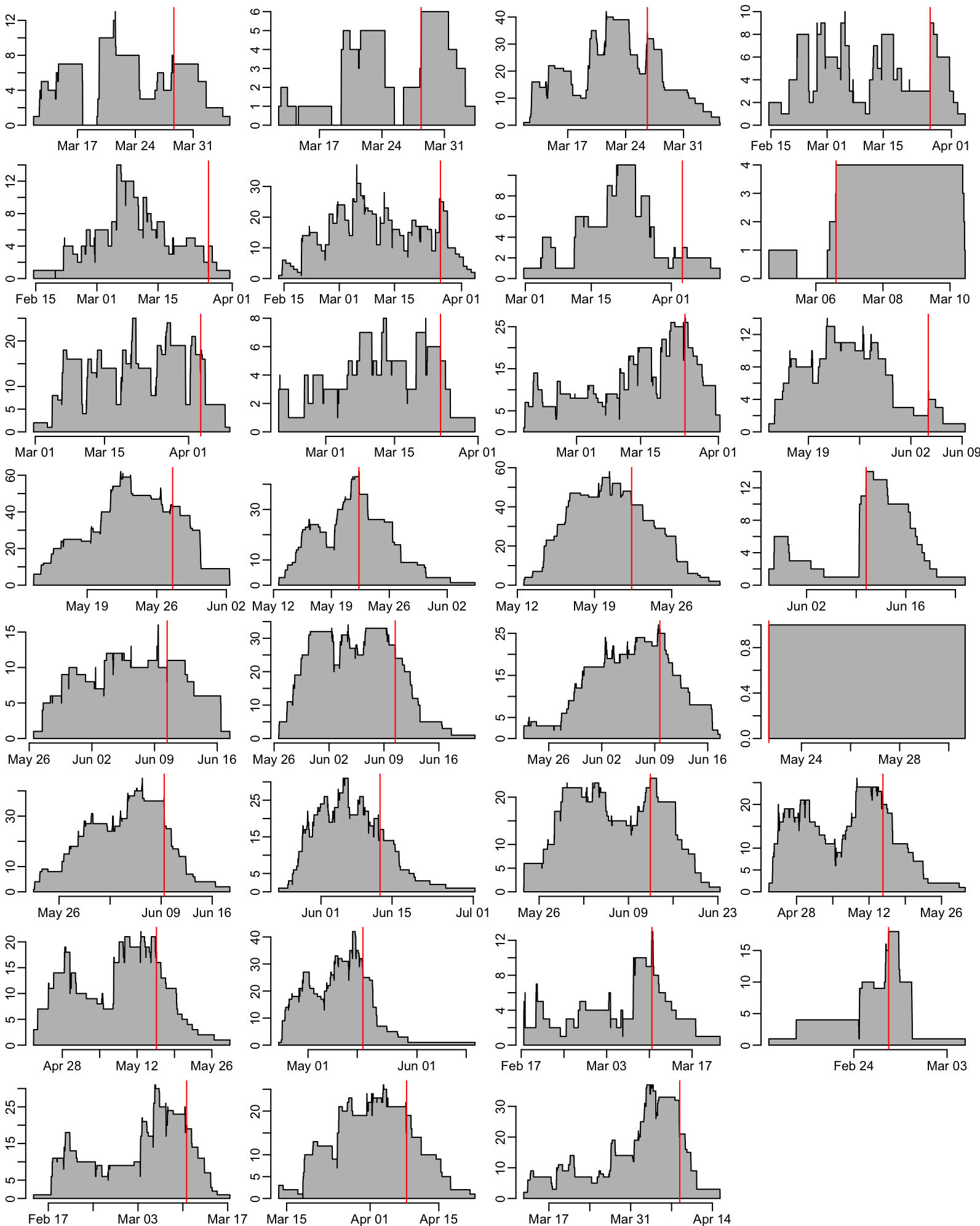
6.4 Durations
The distribution of the durations of stay in the wards:
ward_dates |>
  mutate(duration = as.numeric(DISCHARGE - ADMISSION) / mpd) |>
  pull(duration) |>
  hist2(xlab = "duration of stay (days)", ylab = "number of patients")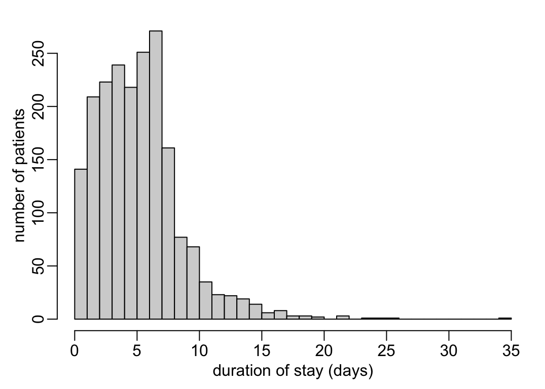
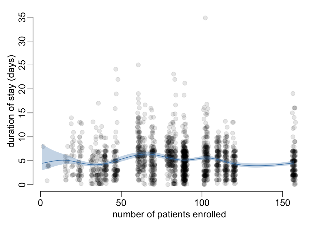
Let’s see whether there any trend on the duration of stay across wards:
the_data <- ward_dates |>
  mutate(duration = as.numeric(DISCHARGE - ADMISSION) / mpd) |>
  left_join(nb_wards, "ward") |>
  select(n, duration)

the_model <- gam(duration ~ s(n), Gamma, the_data, method = "REML") |>
  fitted_values(tibble(n = seq(min(the_data$n), max(the_data$n), le = 512)))

with(the_data, plot(jitter(n, 5), duration, col = adjustcolor("black", .1), pch = 19,
                    xlab = "number of patients enrolled",
                    ylab = "duration of stay (days)"))

color_model <- "steelblue"
with(the_model, {
  polygon2(n, .lower_ci, .upper_ci, col = adjustcolor(color_model, .3))
  lines(n, .fitted, col = color_model)
})
7 MALDI-TOF data
List of genus to exclude:
genus2exclude <- c("Aeromonas", "Enterococcus", "Acinetobacter", "Cupriavidus",
                   "Pseudomonas")
Reading the MALDI-TOF data:
(MALDITOF <- path2data |>
  paste0(MALDITOF_file) |>
  read_excel() |>
  select(USUBJID, SampleSchedule, Identification_MALDITOF) |>
  unique() |>
  mutate(binom_name = Identification_MALDITOF) |>
  separate_wider_delim(binom_name, " ", names = c("genus", "species")) |>
  filter(! genus %in% genus2exclude))
# A tibble: 1,146 × 5
USUBJID SampleSchedule Identification_MALDITOF genus species
<chr> <chr> <chr> <chr> <chr>
1 010-1-1-01 ADMISSION Klebsiella pneumoniae Klebsiella pneumoniae
2 160-1-1-09 ADMISSION Enterobacter hormaechei Enterobacter hormaechei
3 160-2-1-06 ADMISSION Klebsiella pneumoniae Klebsiella pneumoniae
4 160-2-1-04 ADMISSION Enterobacter hormaechei Enterobacter hormaechei
5 160-2-1-04 DISCHARGE Enterobacter hormaechei Enterobacter hormaechei
6 010-1-1-06 DISCHARGE Enterobacter cloacae Enterobacter cloacae
7 010-1-1-01 DISCHARGE Klebsiella pneumoniae Klebsiella pneumoniae
8 010-1-1-14 ADMISSION Klebsiella aerogenes Klebsiella aerogenes
9 160-2-1-06 DISCHARGE Klebsiella pneumoniae Klebsiella pneumoniae
10 010-1-1-03 DISCHARGE Klebsiella pneumoniae Klebsiella pneumoniae
# ℹ 1,136 more rowsThe list of positive samples:
(MALDITOF_samples <- MALDITOF |>
  select(- Identification_MALDITOF) |>
  unique())
# A tibble: 1,146 × 4
USUBJID SampleSchedule genus species
<chr> <chr> <chr> <chr>
1 010-1-1-01 ADMISSION Klebsiella pneumoniae
2 160-1-1-09 ADMISSION Enterobacter hormaechei
3 160-2-1-06 ADMISSION Klebsiella pneumoniae
4 160-2-1-04 ADMISSION Enterobacter hormaechei
5 160-2-1-04 DISCHARGE Enterobacter hormaechei
6 010-1-1-06 DISCHARGE Enterobacter cloacae
7 010-1-1-01 DISCHARGE Klebsiella pneumoniae
8 010-1-1-14 ADMISSION Klebsiella aerogenes
9 160-2-1-06 DISCHARGE Klebsiella pneumoniae
10 010-1-1-03 DISCHARGE Klebsiella pneumoniae
# ℹ 1,136 more rowsThe number of positive samples at admission is:
(nb_positive_samples_admission <- MALDITOF_samples |>
  filter(SampleSchedule == "ADMISSION") |>
  nrow())
[1] 388The number of positive samples at discharge is:
(nb_positive_samples_discharge <- MALDITOF_samples |>
  filter(SampleSchedule == "DISCHARGE") |>
  nrow())
[1] 758The number of positive samples is:
(nb_positive_samples <- nb_positive_samples_admission + nb_positive_samples_discharge)[1] 1146Which represents 29.35 % of samples. The distribution of bacteria across the samples:
prevalences <- function(x, nb_positive_samples, nb_samples) {
  x |>
    group_by(Identification_MALDITOF) |>
    tally() |>
    mutate(`% +ve smpls` = round(100 * n / nb_positive_samples, 1),
           `% all smpls` = round(100 * n / nb_samples, 1)) |>
    arrange(desc(n))
}
Prevalences across all samples:
(prevalences_all <- prevalences(MALDITOF, nb_positive_samples, nb_samples))# A tibble: 16 × 4
Identification_MALDITOF n `% +ve smpls` `% all smpls`
<chr> <int> <dbl> <dbl>
1 Escherichia coli 828 72.3 21.2
2 Klebsiella pneumoniae 189 16.5 4.8
3 Enterobacter hormaechei 72 6.3 1.8
4 Enterobacter cloacae 24 2.1 0.6
5 Klebsiella aerogenes 10 0.9 0.3
6 Citrobacter freundii 6 0.5 0.2
7 Enterobacter kobei 4 0.3 0.1
8 Raoultella ornithinolytica 3 0.3 0.1
9 Escherichia hermannii 2 0.2 0.1
10 Kluyvera georgiana 2 0.2 0.1
11 Citrobacter braakii 1 0.1 0
12 Cronobacter sp. 1 0.1 0
13 Enterobacter bugandensis 1 0.1 0
14 Enterobacter roggenkampii 1 0.1 0
15 Klebsiella oxytoca 1 0.1 0
16 Klebsiella variicola 1 0.1 0 The list of all the bacteria in the MALDITOF results:
(bugs <- prevalences_all |>
  filter(Identification_MALDITOF != "unidentified") |>
  pull(Identification_MALDITOF) |>
  sort())
[1] "Citrobacter braakii" "Citrobacter freundii"
[3] "Cronobacter sp." "Enterobacter bugandensis"
[5] "Enterobacter cloacae" "Enterobacter hormaechei"
[7] "Enterobacter kobei" "Enterobacter roggenkampii"
[9] "Escherichia coli" "Escherichia hermannii"
[11] "Klebsiella aerogenes" "Klebsiella oxytoca"
[13] "Klebsiella pneumoniae" "Klebsiella variicola"
[15] "Kluyvera georgiana" "Raoultella ornithinolytica"Prevalences at admission:
(prevalences_admission <- MALDITOF |>
  filter(SampleSchedule == "ADMISSION") |>
  prevalences(nb_positive_samples_admission, nb_samples_admission))
# A tibble: 8 × 4
Identification_MALDITOF n `% +ve smpls` `% all smpls`
<chr> <int> <dbl> <dbl>
1 Escherichia coli 305 78.6 15.2
2 Klebsiella pneumoniae 56 14.4 2.8
3 Enterobacter hormaechei 17 4.4 0.8
4 Klebsiella aerogenes 4 1 0.2
5 Enterobacter cloacae 3 0.8 0.1
6 Enterobacter bugandensis 1 0.3 0
7 Enterobacter kobei 1 0.3 0
8 Escherichia hermannii 1 0.3 0 Prevalences at discharge:
(prevalences_discharge <- MALDITOF |>
  filter(SampleSchedule == "DISCHARGE") |>
  prevalences(nb_positive_samples_discharge, nb_samples_discharge))
# A tibble: 15 × 4
Identification_MALDITOF n `% +ve smpls` `% all smpls`
<chr> <int> <dbl> <dbl>
1 Escherichia coli 523 69 27.5
2 Klebsiella pneumoniae 133 17.5 7
3 Enterobacter hormaechei 55 7.3 2.9
4 Enterobacter cloacae 21 2.8 1.1
5 Citrobacter freundii 6 0.8 0.3
6 Klebsiella aerogenes 6 0.8 0.3
7 Enterobacter kobei 3 0.4 0.2
8 Raoultella ornithinolytica 3 0.4 0.2
9 Kluyvera georgiana 2 0.3 0.1
10 Citrobacter braakii 1 0.1 0.1
11 Cronobacter sp. 1 0.1 0.1
12 Enterobacter roggenkampii 1 0.1 0.1
13 Escherichia hermannii 1 0.1 0.1
14 Klebsiella oxytoca 1 0.1 0.1
15 Klebsiella variicola 1 0.1 0.1Let’s compare the prevalences at admission and discharge:
prev_adm_disch <- prevalences_all |>
  select(Identification_MALDITOF) |>
  left_join(prevalences_admission, "Identification_MALDITOF") |>
  left_join(prevalences_discharge, "Identification_MALDITOF",
            suffix = c(" (A)", " (D)")) |>
  mutate(across(everything(), ~ replace_na(.x, 0)))
The number of positive samples:
prev_adm_disch |>
  select(Identification_MALDITOF, starts_with("n"))
# A tibble: 16 × 3
Identification_MALDITOF `n (A)` `n (D)`
<chr> <int> <int>
1 Escherichia coli 305 523
2 Klebsiella pneumoniae 56 133
3 Enterobacter hormaechei 17 55
4 Enterobacter cloacae 3 21
5 Klebsiella aerogenes 4 6
6 Citrobacter freundii 0 6
7 Enterobacter kobei 1 3
8 Raoultella ornithinolytica 0 3
9 Escherichia hermannii 1 1
10 Kluyvera georgiana 0 2
11 Citrobacter braakii 0 1
12 Cronobacter sp. 0 1
13 Enterobacter bugandensis 1 0
14 Enterobacter roggenkampii 0 1
15 Klebsiella oxytoca 0 1
16 Klebsiella variicola 0 1Their proportion among positive samples:
prev_adm_disch |>
  select(Identification_MALDITOF, starts_with("% +"))
# A tibble: 16 × 3
Identification_MALDITOF `% +ve smpls (A)` `% +ve smpls (D)`
<chr> <dbl> <dbl>
1 Escherichia coli 78.6 69
2 Klebsiella pneumoniae 14.4 17.5
3 Enterobacter hormaechei 4.4 7.3
4 Enterobacter cloacae 0.8 2.8
5 Klebsiella aerogenes 1 0.8
6 Citrobacter freundii 0 0.8
7 Enterobacter kobei 0.3 0.4
8 Raoultella ornithinolytica 0 0.4
9 Escherichia hermannii 0.3 0.1
10 Kluyvera georgiana 0 0.3
11 Citrobacter braakii 0 0.1
12 Cronobacter sp. 0 0.1
13 Enterobacter bugandensis 0.3 0
14 Enterobacter roggenkampii 0 0.1
15 Klebsiella oxytoca 0 0.1
16 Klebsiella variicola 0 0.1Their proportions among all samples:
prev_adm_disch |>
  select(Identification_MALDITOF, starts_with("% a"))
# A tibble: 16 × 3
Identification_MALDITOF `% all smpls (A)` `% all smpls (D)`
<chr> <dbl> <dbl>
1 Escherichia coli 15.2 27.5
2 Klebsiella pneumoniae 2.8 7
3 Enterobacter hormaechei 0.8 2.9
4 Enterobacter cloacae 0.1 1.1
5 Klebsiella aerogenes 0.2 0.3
6 Citrobacter freundii 0 0.3
7 Enterobacter kobei 0 0.2
8 Raoultella ornithinolytica 0 0.2
9 Escherichia hermannii 0 0.1
10 Kluyvera georgiana 0 0.1
11 Citrobacter braakii 0 0.1
12 Cronobacter sp. 0 0.1
13 Enterobacter bugandensis 0 0
14 Enterobacter roggenkampii 0 0.1
15 Klebsiella oxytoca 0 0.1
16 Klebsiella variicola 0 0.1The list of bacteria absent at admission and present at discharge:
prev_adm_disch |>
  select(Identification_MALDITOF, starts_with("n")) |>
  filter(`n (A)` == 0)
# A tibble: 8 × 3
Identification_MALDITOF `n (A)` `n (D)`
<chr> <int> <int>
1 Citrobacter freundii 0 6
2 Raoultella ornithinolytica 0 3
3 Kluyvera georgiana 0 2
4 Citrobacter braakii 0 1
5 Cronobacter sp. 0 1
6 Enterobacter roggenkampii 0 1
7 Klebsiella oxytoca 0 1
8 Klebsiella variicola 0 1The list of bacteria present at admission and absent at discharge:
prev_adm_disch |>
  select(Identification_MALDITOF, starts_with("n")) |>
  filter(`n (D)` == 0)
# A tibble: 1 × 3
Identification_MALDITOF `n (A)` `n (D)`
<chr> <int> <int>
1 Enterobacter bugandensis 1 0Let’s now look at changes in colonization status between admission and discharge. The following function prepares the data for an alluvial plot:
make_alluvial_data <- function(x) {
  positive_samples <- x |>
    mutate(state = 2) |> # the exact value here does not matter
    pivot_wider(names_from = SampleSchedule, values_from = state) |>
    mutate(across(-USUBJID, ~ ! is.na(.x)))

  dates |>
    filter(! is.na(DISCHARGE)) |>
    select(USUBJID) |>
    left_join(positive_samples, "USUBJID") |>
    mutate(across(-USUBJID, ~ replace_na(.x, FALSE)),
           across(-USUBJID, ~ c("cleared", "colonized")[as.numeric(.x) + 1])) |>
    group_by(ADMISSION, DISCHARGE) |>
    tally() |>
    ungroup()
}
The following function is a wrapper around the above function and the the alluvial3() function that computes the table of changes and plot the alluvial plot for a given set of bacteria to consider:
plot_changes <- function(bacteria = "all") {
  if (bacteria == "all") {
    the_data <- MALDITOF_samples
  } else {
    the_data <- MALDITOF |>
           filter(Identification_MALDITOF %in% bacteria) |>
           select(- Identification_MALDITOF)
  }
  the_data |>
    make_alluvial_data() |>
    alluvial3(col = "grey", alpha = .8, border = NA)
}
Let’s use this function to look at some example:
plot_changes()# A tibble: 4 × 3
ADMISSION DISCHARGE n
<chr> <chr> <int>
1 cleared cleared 1122
2 cleared colonized 524
3 colonized cleared 142
4 colonized colonized 234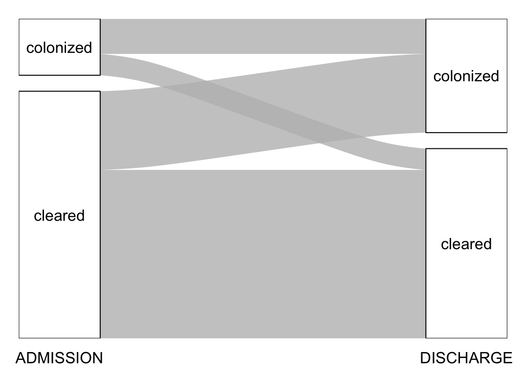
plot_changes("Escherichia coli")# A tibble: 4 × 3
ADMISSION DISCHARGE n
<chr> <chr> <int>
1 cleared cleared 1290
2 cleared colonized 317
3 colonized cleared 91
4 colonized colonized 206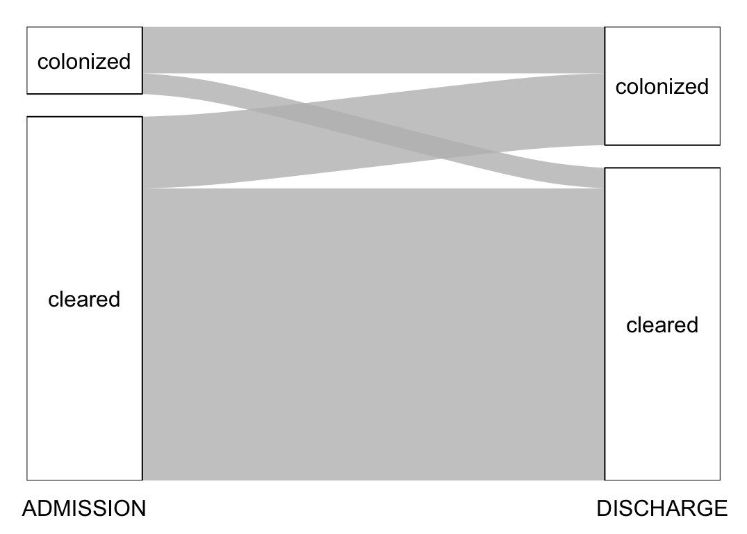
plot_changes("Klebsiella pneumoniae")# A tibble: 4 × 3
ADMISSION DISCHARGE n
<chr> <chr> <int>
1 cleared cleared 1739
2 cleared colonized 110
3 colonized cleared 32
4 colonized colonized 23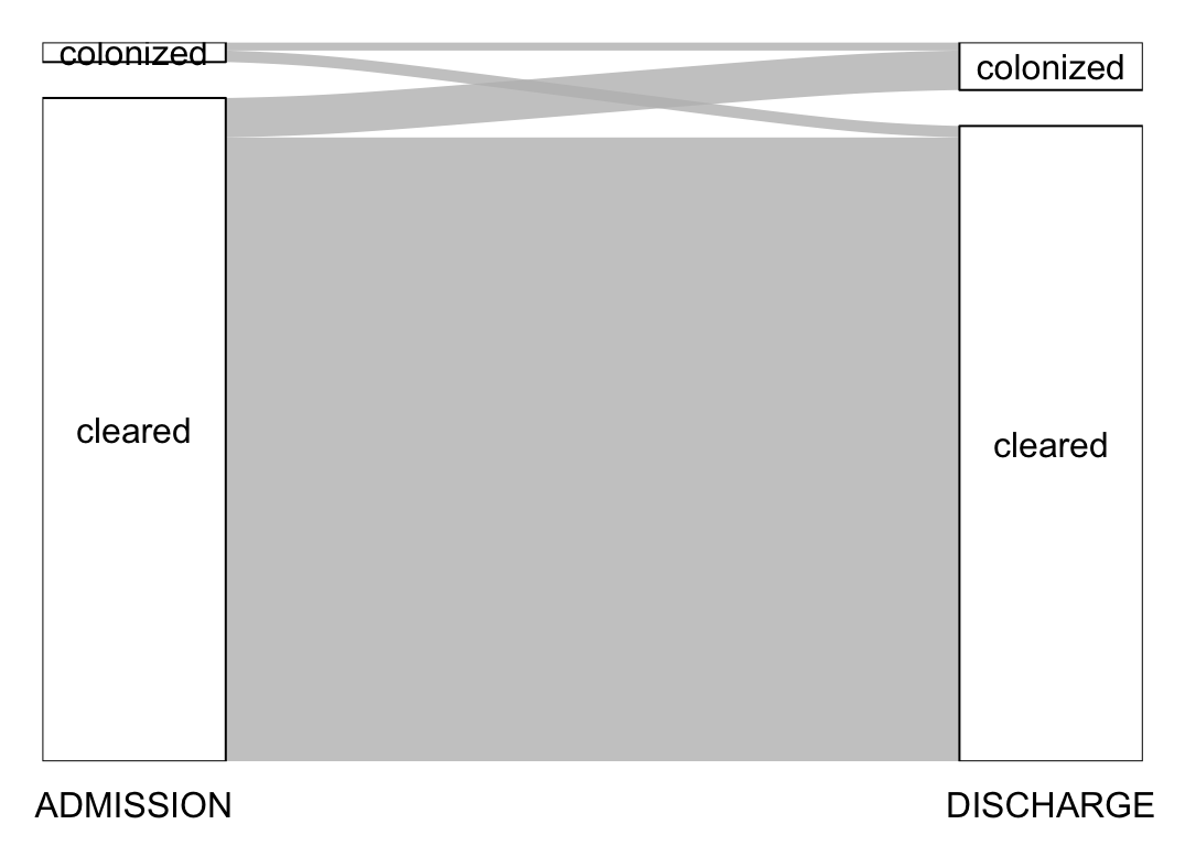
8 CRE exposure
8.1 All CRE
The number of enrolled patient with CRE at admission as a function of time for each ward (takes 1.5”):
opar <- par(mfrow = c(8, 4))

CRE_admission <- MALDITOF_samples |>
  filter(SampleSchedule == "ADMISSION") |>
  pull(USUBJID)

ward_dates |>
  filter(USUBJID %in% CRE_admission) |>
  group_by(ward) |>
  group_map(~ ward_occupancy(.x), .keep = TRUE) |>
  walk(plot_occ, ann = FALSE)

par(opar)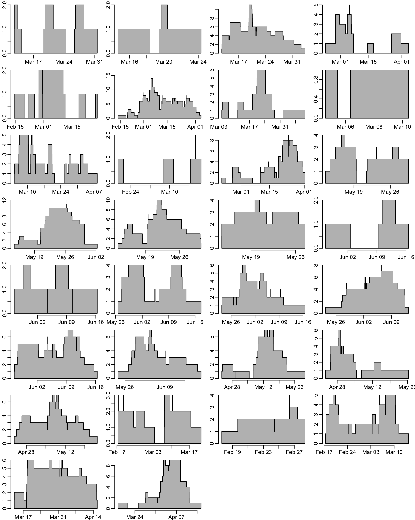
A function that plots the prevalence estimate estimate and lower and upper bonds lower and upper of the confidence interval from a data frame of a ward:
plot_prevalence <- function(x) {
  with(x, plot(x_transform(date), y_transform(estimate),
               type = "n", ann = FALSE, ylim = 0:1))
  x |>
    duplicate_NA_rows() |>
    remove_NAs(estimate) |>
    map(~ with(.x, polygon2(x_transform(date), y_transform(lower), y_transform(upper),
                            col = "grey")))
  with(x, lines(x_transform(date), y_transform(estimate)))
}
Computing the proportions of CRE positives as a function of time for each ward (takes 1.5”):
numerator_df <- ward_dates |>
  filter(USUBJID %in% CRE_admission) |>
  group_by(ward) |>
  group_modify(~ ward_occupancy(.x)) |>
  rename(numerator = occupancy)

proportion_CRE <- ward_dates |>
  group_by(ward) |>
  group_modify(~ ward_occupancy(.x)) |>
  ungroup() |>
  rename(denominator = occupancy) |>
  left_join(numerator_df, c("ward", "date")) |>
  fill(numerator) |>
  mutate(across(numerator, ~ replace_na(.x, 0)),
         Clopper_Pearson = map2(numerator, denominator, binom_test)) |>
  unnest_wider(Clopper_Pearson)
Proportion of enrolled patients that are CRE positive at admission as a function of time for each ward (takes 1.5”):
opar <- par(mfrow = c(8, 4))
proportion_CRE |>
  group_by(ward) |>
  group_walk(~ plot_prevalence(.x))
par(opar)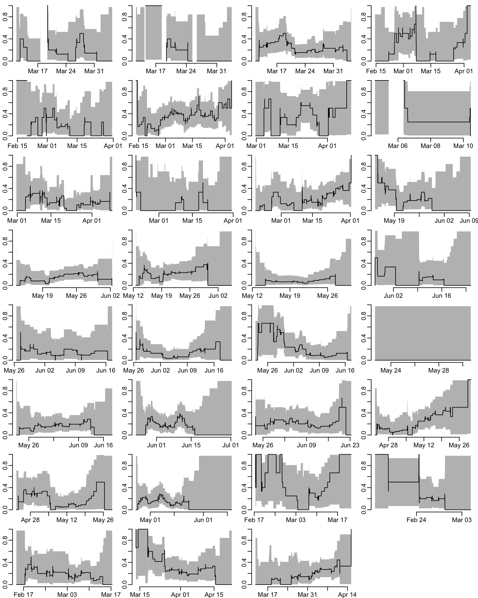
8.2 K. pneumoniae
Here we have the same plots as for the previous section but for K. pneumoniae only. First the number of enrolled patient with CRE K. pneumoniae at admission as a function of time for each ward (takes 1”):
opar <- par(mfrow = c(8, 4))

Kp_admission <- MALDITOF |>
  filter(SampleSchedule == "ADMISSION",
         Identification_MALDITOF == "Klebsiella pneumoniae") |>
  pull(USUBJID)

ward_dates |>
  filter(USUBJID %in% Kp_admission) |>
  group_by(ward) |>
  group_map(~ ward_occupancy(.x), .keep = TRUE) |>
  walk(plot_occ, ann = FALSE)

par(opar)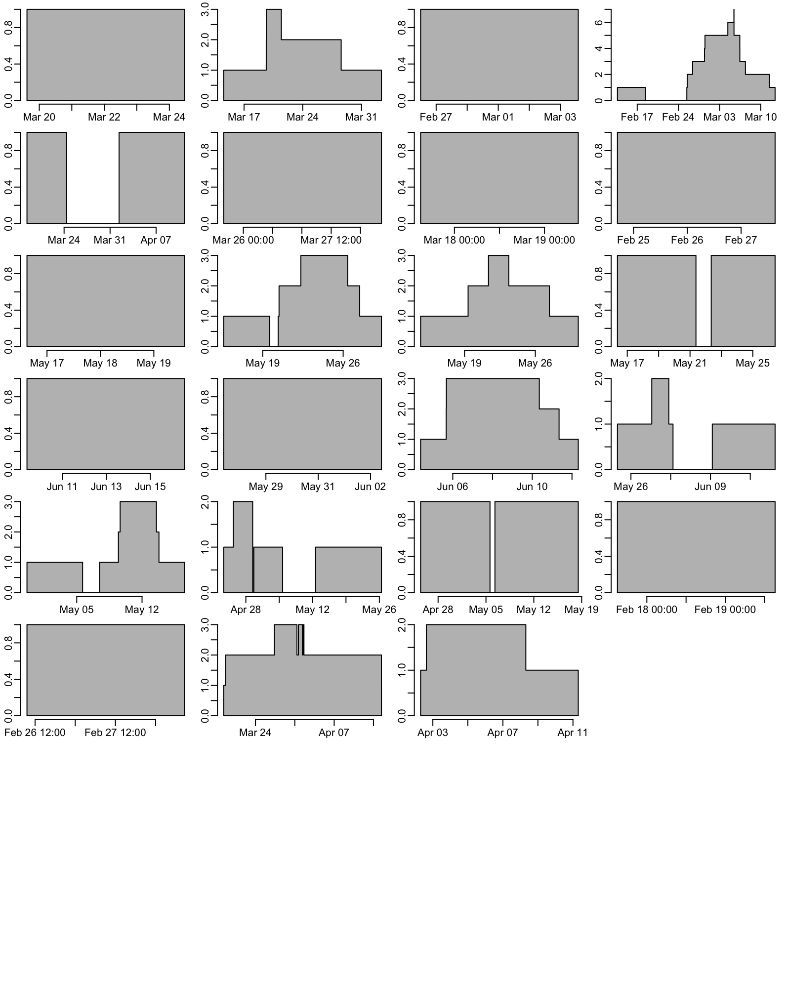
Proportion of enrolled patients that are CRE K. pneumoniae positive at admission as a function of time for each ward (takes 1.5”):
numerator_df <- ward_dates |>
  filter(USUBJID %in% Kp_admission) |>
  group_by(ward) |>
  group_modify(~ ward_occupancy(.x)) |>
  rename(numerator = occupancy)

opar <- par(mfrow = c(8, 4))

ward_dates |>
  group_by(ward) |>
  group_modify(~ ward_occupancy(.x)) |>
  ungroup() |>
  rename(denominator = occupancy) |>
  left_join(numerator_df, c("ward", "date")) |>
  fill(numerator) |>
  mutate(across(numerator, ~ replace_na(.x, 0)),
         Clopper_Pearson = map2(numerator, denominator, binom_test)) |>
  unnest_wider(Clopper_Pearson) |>
  group_by(ward) |>
  group_walk(~ plot_prevalence(.x))

par(opar)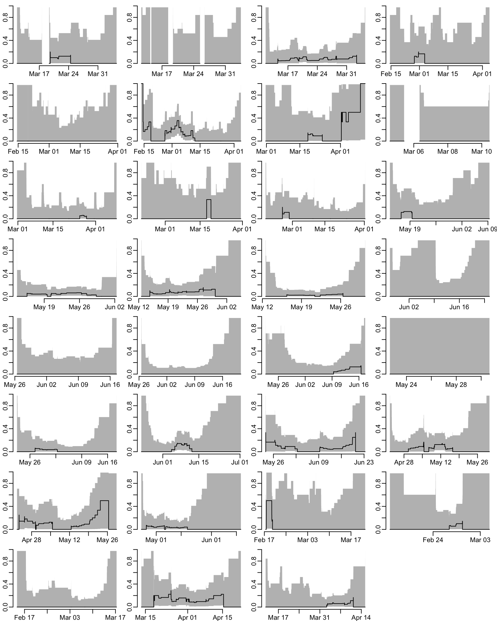
9 Data preparation
9.1 Minimum data
A function that generates the presence/absence data (coded as 2/1 here) from the output x of the MALDITOF where id is the column of x that contains the patient ID, time_point is the column of x that contains the time point of the sample (e.g. ADMISSION or DISCHARGE), identification is the column of x that contains the bacteria identified by the MALDITOF and bacteria is a vector of characters that contains the names of the bacteria that we want to test the presence of.
presence_abscence <- function(x, id, time_point, identification, bacteria) {
  x |>
    group_by({{ id }}, {{ time_point }}) |>
    group_modify(~ col2listcol(.x, {{ identification }})) |>
    ungroup() |>
    mutate(state = map_lgl({{ identification }}, ~ any(bacteria %in% .x)) + 1) |>
    select(- {{ identification }}) |>
    arrange({{ id }}, {{ time_point }})
}
The following function adds the samples that were tested negative to the output x of presence_abscence() where y is the samples dates as generated in Section 6.1.
add_negatives <- function(x, y, id, time_point) {
  tp <- as_name(enquo(time_point))
  y |>
    pivot_longer(- {{ id }}, names_to = tp) |>
    left_join(x, c(as_name(enquo(id)), tp)) |>
    mutate(across(state, ~ replace_na(., 1)))
}
A function that selects patients from x who have samples from at least 2 time points:
select2time_points <- function(x, id) {
  id_with_2obs <- x |>
    filter_out(is.na(value)) |>
    pull({{ id }}) |>
    table() |>
    is_greater_than(1) |>
    which() |>
    names()

  filter(x, {{ id }} %in% id_with_2obs)
}
where id is the column of x that contains the patients IDs. A function that combines state and time data:
state_time <- function(state, time, id, admission, discharge, time_point) {
  time |>
    mutate("{{discharge}}" := as.numeric({{ discharge }} - {{ admission }}) / mpd,
           "{{admission}}" := 0) |>
    pivot_longer(- {{ id }},
                 names_to = as_name(enquo(time_point)), values_to = "days") |>
    left_join(x = {{ state }}, y = _,
              c(as_name(enquo(id)), as_name(enquo(time_point))))
}
The following function puts the 4 above functions together:
msm_data <- function(x, y, id, time_point, identification, bacteria,
                     admission, discharge) {
  x |>
    presence_abscence({{ id }}, {{ time_point }}, {{ identification }}, bacteria) |>
    add_negatives(y, {{ id }}, {{ time_point }}) |>
    select2time_points({{ id }}) |>
    state_time(y, {{ id }}, {{ admission }}, {{ discharge }}, {{ time_point }}) |>
    select({{ id }}, state, days)
}
where
xis the MALDITOF data as read in section Section 7yis the dates of samples collections as generated from the CRF in section Section 6.1idis the unquoted name of the patient ID variable that should be the same inxandytime_pointis the unquoted name of the variable ofxthat contains the time point information (for exampleADMISSIONandDISCHARGE)identificationis the unquoted name of the variable ofxthat contains the name of the identified bacteriabacteriais a vector of quoted names of bacteria we want to generate the data foradmissionis the unquoted name of the variable ofythat contains the dates of admissionsdischargeis the unquoted name of the variable ofythat contains the dates of discharge
The output of this function is a data frame with 3 columns:
- the
idpatient ID - the
statevariable, with1and2for not “not infected” and “infected” respectively - the
dayscolumns where zeros refers to admissions and non-zero values are the times of discharge in days counting from admission
A tuning of msm_data():
msm_data2 <- function(bacteria) msm_data(MALDITOF, dates, USUBJID, SampleSchedule,
                                         Identification_MALDITOF, bacteria, ADMISSION,
                                         DISCHARGE)
9.2 Covariates
The following function adds to the output x of the msm_data() function the covariate otherCRE that tells whether at admission the patient had a CRE other than the set of bacteria:
add_other_CRE_at_admission <- function(x, bacteria) {
  MALDITOF |>
    filter(SampleSchedule == "ADMISSION",
           ! Identification_MALDITOF %in% bacteria) |>
    mutate(otherCRE = TRUE) |>
    select(USUBJID, otherCRE) |>
    unique() |>
    left_join(x = x, y = _, "USUBJID") |>
    mutate(across(otherCRE, ~ replace_na(.x, FALSE)))
}
This function relies on the MALDITOF data frame generated in section Section 7. The following function adds to the output x of the msm_data() function the ward ID covariate:
add_ward <- function(x) left_join(x, wards, "USUBJID")This function relies on the wards data frame generated in the section Section 6.2. The following function adds to the output x of the add_ward() function the covariates estimate, lower and upper that are the temporal means of the proportions of enrolled patient that are CRE positive in the ward for the duration of the study:
add_CRE_prevalence_in_ward <- function(x) {
  ward_means <- function(y) {
    total_duration <- time_diff(range(y$date))
    y |>
      mutate(weight = time_diff(c(date, NA)) / total_duration) |>
      summarise(across(c(estimate, lower, upper),
                       ~ sum(replace_na(.x, 0) * weight, na.rm = TRUE)))
  }
  proportion_CRE |>
    group_by(ward) |>
    group_modify(~ ward_means(.x)) |>
    ungroup() |>
    left_join(x = x, y = _, "ward")
}
This function relies on the proportion_CRE data frame generated in the section Section 8.1.
10 K. pneumoniae
10.1 Preparing the data
Generating the presence/absence of K. pneumoniae (takes 2.5”):
K_pneumoniae_raw <- presence_abscence(MALDITOF, USUBJID, SampleSchedule,
                                      Identification_MALDITOF, "Klebsiella pneumoniae")
Which gives:
K_pneumoniae_raw# A tibble: 1,038 × 5
USUBJID SampleSchedule genus species state
<chr> <chr> <chr> <chr> <dbl>
1 008-1-1-05 ADMISSION Escherichia coli 1
2 008-1-1-05 DISCHARGE Klebsiella pneumoniae 2
3 008-1-1-07 ADMISSION Escherichia coli 1
4 008-1-1-07 DISCHARGE Escherichia coli 1
5 008-1-1-08 ADMISSION Escherichia coli 1
6 008-1-1-08 DISCHARGE Escherichia coli 1
7 008-1-1-100 DISCHARGE Enterobacter hormaechei 1
8 008-1-1-14 ADMISSION Escherichia coli 1
9 008-1-1-14 DISCHARGE Kluyvera georgiana 1
10 008-1-1-15 DISCHARGE Escherichia coli 1
# ℹ 1,028 more rowsWhere 1 is absence and 2 is presence. Adding the samples with negative culture:
(K_pneumoniae_raw_a <- add_negatives(K_pneumoniae_raw, dates, USUBJID, SampleSchedule))# A tibble: 4,000 × 6
USUBJID SampleSchedule value genus species state
<chr> <chr> <dttm> <chr> <chr> <dbl>
1 008-1-1-01 ADMISSION 2025-03-11 16:30:00 <NA> <NA> 1
2 008-1-1-01 DISCHARGE 2025-03-13 14:40:00 <NA> <NA> 1
3 008-1-1-02 ADMISSION 2025-03-12 10:00:00 <NA> <NA> 1
4 008-1-1-02 DISCHARGE 2025-03-14 10:00:00 <NA> <NA> 1
5 008-1-1-03 ADMISSION 2025-03-12 09:50:00 <NA> <NA> 1
6 008-1-1-03 DISCHARGE 2025-03-14 09:50:00 <NA> <NA> 1
7 008-1-1-04 ADMISSION 2025-03-12 13:45:00 <NA> <NA> 1
8 008-1-1-04 DISCHARGE 2025-03-13 14:55:00 <NA> <NA> 1
9 008-1-1-05 ADMISSION 2025-03-12 13:40:00 Escherichia coli 1
10 008-1-1-05 DISCHARGE 2025-03-28 17:00:00 Klebsiella pneumoniae 2
# ℹ 3,990 more rowsSelecting the patients that have samples from at least 2 time points:
(K_pneumoniae <- select2time_points(K_pneumoniae_raw_a, USUBJID))# A tibble: 3,808 × 6
USUBJID SampleSchedule value genus species state
<chr> <chr> <dttm> <chr> <chr> <dbl>
1 008-1-1-01 ADMISSION 2025-03-11 16:30:00 <NA> <NA> 1
2 008-1-1-01 DISCHARGE 2025-03-13 14:40:00 <NA> <NA> 1
3 008-1-1-02 ADMISSION 2025-03-12 10:00:00 <NA> <NA> 1
4 008-1-1-02 DISCHARGE 2025-03-14 10:00:00 <NA> <NA> 1
5 008-1-1-03 ADMISSION 2025-03-12 09:50:00 <NA> <NA> 1
6 008-1-1-03 DISCHARGE 2025-03-14 09:50:00 <NA> <NA> 1
7 008-1-1-04 ADMISSION 2025-03-12 13:45:00 <NA> <NA> 1
8 008-1-1-04 DISCHARGE 2025-03-13 14:55:00 <NA> <NA> 1
9 008-1-1-05 ADMISSION 2025-03-12 13:40:00 Escherichia coli 1
10 008-1-1-05 DISCHARGE 2025-03-28 17:00:00 Klebsiella pneumoniae 2
# ℹ 3,798 more rowsMaking the dataset for the multistate modelling:
(Kp_msm <- state_time(K_pneumoniae, dates, USUBJID,
                      ADMISSION, DISCHARGE, SampleSchedule))
# A tibble: 3,808 × 7
USUBJID SampleSchedule value genus species state days
<chr> <chr> <dttm> <chr> <chr> <dbl> <dbl>
1 008-1-1-01 ADMISSION 2025-03-11 16:30:00 <NA> <NA> 1 0
2 008-1-1-01 DISCHARGE 2025-03-13 14:40:00 <NA> <NA> 1 1.92
3 008-1-1-02 ADMISSION 2025-03-12 10:00:00 <NA> <NA> 1 0
4 008-1-1-02 DISCHARGE 2025-03-14 10:00:00 <NA> <NA> 1 2
5 008-1-1-03 ADMISSION 2025-03-12 09:50:00 <NA> <NA> 1 0
6 008-1-1-03 DISCHARGE 2025-03-14 09:50:00 <NA> <NA> 1 2
7 008-1-1-04 ADMISSION 2025-03-12 13:45:00 <NA> <NA> 1 0
8 008-1-1-04 DISCHARGE 2025-03-13 14:55:00 <NA> <NA> 1 1.05
9 008-1-1-05 ADMISSION 2025-03-12 13:40:00 Escherichia coli 1 0
10 008-1-1-05 DISCHARGE 2025-03-28 17:00:00 Klebsiella pneumo… 2 16.1
# ℹ 3,798 more rowsAlternatively, we can do all at once with this function (takes 2.5”):
Kp_msm <- msm_data(MALDITOF, dates, USUBJID, SampleSchedule, Identification_MALDITOF,
                   "Klebsiella pneumoniae", ADMISSION, DISCHARGE)
which gives:
Kp_msm# A tibble: 3,808 × 3
USUBJID state days
<chr> <dbl> <dbl>
1 008-1-1-01 1 0
2 008-1-1-01 1 1.92
3 008-1-1-02 1 0
4 008-1-1-02 1 2
5 008-1-1-03 1 0
6 008-1-1-03 1 2
7 008-1-1-04 1 0
8 008-1-1-04 1 1.05
9 008-1-1-05 1 0
10 008-1-1-05 2 16.1
# ℹ 3,798 more rowsOr, even simpler here (takes 2.5”):
Kp_msm <- msm_data2("Klebsiella pneumoniae")Adding covariates:
(Kp_msm_cov <- Kp_msm |>
   add_other_CRE_at_admission("Klebsiella pneumoniae") |>
   add_ward() |>
   add_CRE_prevalence_in_ward())
# A tibble: 3,808 × 8
USUBJID state days otherCRE ward estimate lower upper
<chr> <dbl> <dbl> <lgl> <chr> <dbl> <dbl> <dbl>
1 008-1-1-01 1 0 FALSE 008100 0.231 0.0757 0.538
2 008-1-1-01 1 1.92 FALSE 008100 0.231 0.0757 0.538
3 008-1-1-02 1 0 FALSE 008100 0.231 0.0757 0.538
4 008-1-1-02 1 2 FALSE 008100 0.231 0.0757 0.538
5 008-1-1-03 1 0 FALSE 008100 0.231 0.0757 0.538
6 008-1-1-03 1 2 FALSE 008100 0.231 0.0757 0.538
7 008-1-1-04 1 0 FALSE 008100 0.231 0.0757 0.538
8 008-1-1-04 1 1.05 FALSE 008100 0.231 0.0757 0.538
9 008-1-1-05 1 0 TRUE 008100 0.231 0.0757 0.538
10 008-1-1-05 2 16.1 TRUE 008100 0.231 0.0757 0.538
# ℹ 3,798 more rows10.2 Multi-state modelling
10.2.1 Basic operations
Defining the structure of the \(Q\) matrix:
Q <- rbind(c(0, 1),
           c(1, 0))
Initial values of the \(Q\) matrix:
(Q_crude <- crudeinits.msm(state ~ days, USUBJID, Q, Kp_msm)) [,1] [,2]
[1,] -0.01144174 0.01144174
[2,] 0.08458290 -0.08458290Fitting a simple model without any covariate:
(Kp_msm_fit <- msm(state ~ days, USUBJID, Kp_msm, Q))
Call:
msm(formula = state ~ days, subject = USUBJID, data = Kp_msm,     qmatrix = Q)

Maximum likelihood estimates

Transition intensities
                  Baseline
State 1 - State 1 -0.01978 (-0.02565,-0.01525)
State 1 - State 2  0.01978 ( 0.01525, 0.02565)
State 2 - State 1  0.16116 ( 0.10848, 0.23944)
State 2 - State 2 -0.16116 (-0.23944,-0.10848)

-2 * log-likelihood:  890.9878
Or we call simply do:
(Kp_msm_fit <- bsm(state ~ days, USUBJID, Kp_msm))
Call:
bsm(formula = state ~ days, subject = USUBJID, data = Kp_msm)

Maximum likelihood estimates

Transition intensities
                  Baseline
State 1 - State 1 -0.01978 (-0.02565,-0.01525)
State 1 - State 2  0.01978 ( 0.01525, 0.02565)
State 2 - State 1  0.16116 ( 0.10848, 0.23944)
State 2 - State 2 -0.16116 (-0.23944,-0.10848)

-2 * log-likelihood:  890.9878
Estimated transition intensity \(Q\) matrix:
qmatrix.msm(Kp_msm_fit) State 1 State 2
State 1 -0.01978 (-0.02565,-0.01525) 0.01978 ( 0.01525, 0.02565)
State 2 0.16116 ( 0.10848, 0.23944) -0.16116 (-0.23944,-0.10848)Estimated transition probability \(P\) matrix per day:
pmatrix.msm(Kp_msm_fit) State 1 State 2
State 1 0.9819097 0.01809029
State 2 0.1474229 0.85257708Estimated mean sojourn times in each transient state:
sojourn.msm(Kp_msm_fit) estimates SE L U
State 1 50.565762 6.708416 38.987920 65.581756
State 2 6.204931 1.253325 4.176419 9.218705Log-likelihood of the model:
logLik(Kp_msm_fit)'log Lik.' -445.4939 (df=2)10.2.2 Bootstrapped CIs
Bootstrapping \(Q\) estimates (1000 samples, takes 42” in parallel on 11 cores):
q_list <- boot.msm(Kp_msm_fit, function(x) qmatrix.msm(x)$estimates, 1000,
                   cores = nb_cores)
Reformating the output into an array of dimension 2, 2, and 1000 (i.e. 2 states and 1000 bootstrap samples):
q_array <- array(unlist(q_list), dim = c(2, 2, 1000))Or we can simply do this instead of the above two successive command lines (takes 42” in parallel on 11 cores):
q_array <- boot_msm(Kp_msm_fit, qmatrix.msm, 1000, cores = nb_cores)The bootstrap estimate of the standard deviation:
apply(q_array, 1:2, sd) [,1] [,2]
[1,] 0.002848985 0.002848985
[2,] 0.038611786 0.038611786Or, equivalently, in a formatted output:
boot_stat(q_array) State 1 State 2
State 1 0.002848985 0.002848985
State 2 0.038611786 0.038611786And with the mean:
boot_stat(q_array, mean) State 1 State 2
State 1 -0.02000294 0.02000294
State 2 0.16525797 -0.16525797Or the median:
boot_stat(q_array, median) State 1 State 2
State 1 -0.01976212 0.01976212
State 2 0.16131963 -0.16131963The bootstrap estimate of the 95% confidence interval:
q_array |>
  apply(1:2, function(x) quantile(x, c(.025, .975))) |>
  aperm(c(1, 3, 2))
, , 1
[,1] [,2]
2.5% -0.02639242 0.01515261
97.5% -0.01515261 0.02639242
, , 2
[,1] [,2]
2.5% 0.1022118 -0.2533253
97.5% 0.2533253 -0.1022118Or, equivalently, in a formatted output:
boot_ci(q_array), , State 1
State 1 State 2
2.5% -0.02639242 0.01515261
97.5% -0.01515261 0.02639242
, , State 2
State 1 State 2
2.5% 0.1022118 -0.2533253
97.5% 0.2533253 -0.102211810.2.3 Covariates
(Kp_msm_cov_fit <- bsm(state ~ days, USUBJID, Kp_msm_cov,
                       covariates = list("1-2" = ~ otherCRE)))
Call:
bsm(formula = state ~ days, subject = USUBJID, data = Kp_msm_cov,     covariates = list(`1-2` = ~otherCRE))

Maximum likelihood estimates
Baselines are with covariates set to their means

Transition intensities with hazard ratios for each covariate
                  Baseline                     otherCRETRUE
State 1 - State 1 -0.01976 (-0.02563,-0.01524)
State 1 - State 2  0.01976 ( 0.01524, 0.02563) 0.95 (0.5634,1.602)
State 2 - State 1  0.16105 ( 0.10843, 0.23922) 1.00
State 2 - State 2 -0.16105 (-0.23922,-0.10843)

-2 * log-likelihood: 890.9503 qmatrix.msm(Kp_msm_cov_fit, covariates=list(otherCRE = FALSE)) State 1 State 2
State 1 -0.01993 (-0.02611,-0.01522) 0.01993 ( 0.01522, 0.02611)
State 2 0.16105 ( 0.10843, 0.23922) -0.16105 (-0.23922,-0.10843)qmatrix.msm(Kp_msm_cov_fit, covariates=list(otherCRE = TRUE)) State 1 State 2
State 1 -0.01993 (-0.02611,-0.01522) 0.01993 ( 0.01522, 0.02611)
State 2 0.16105 ( 0.10843, 0.23922) -0.16105 (-0.23922,-0.10843)(Kp_msm_cov_fit <- bsm(state ~ days, USUBJID, Kp_msm_cov,
covariates = list("1-2" = ~ estimate)))
Call:
bsm(formula = state ~ days, subject = USUBJID, data = Kp_msm_cov,     covariates = list(`1-2` = ~estimate))

Maximum likelihood estimates
Baselines are with covariates set to their means

Transition intensities with hazard ratios for each covariate
                  Baseline                     estimate
State 1 - State 1 -0.01978 (-0.02568,-0.01523)
State 1 - State 2  0.01978 ( 0.01523, 0.02568) 0.9597 (0.1223,7.53)
State 2 - State 1  0.16125 ( 0.10848, 0.23969) 1.0000
State 2 - State 2 -0.16125 (-0.23969,-0.10848)

-2 * log-likelihood:  890.9862
10.2.4 Diagnostics
plot.prevalence.msm(Kp_msm_fit, mintime = 0, maxtime = 15)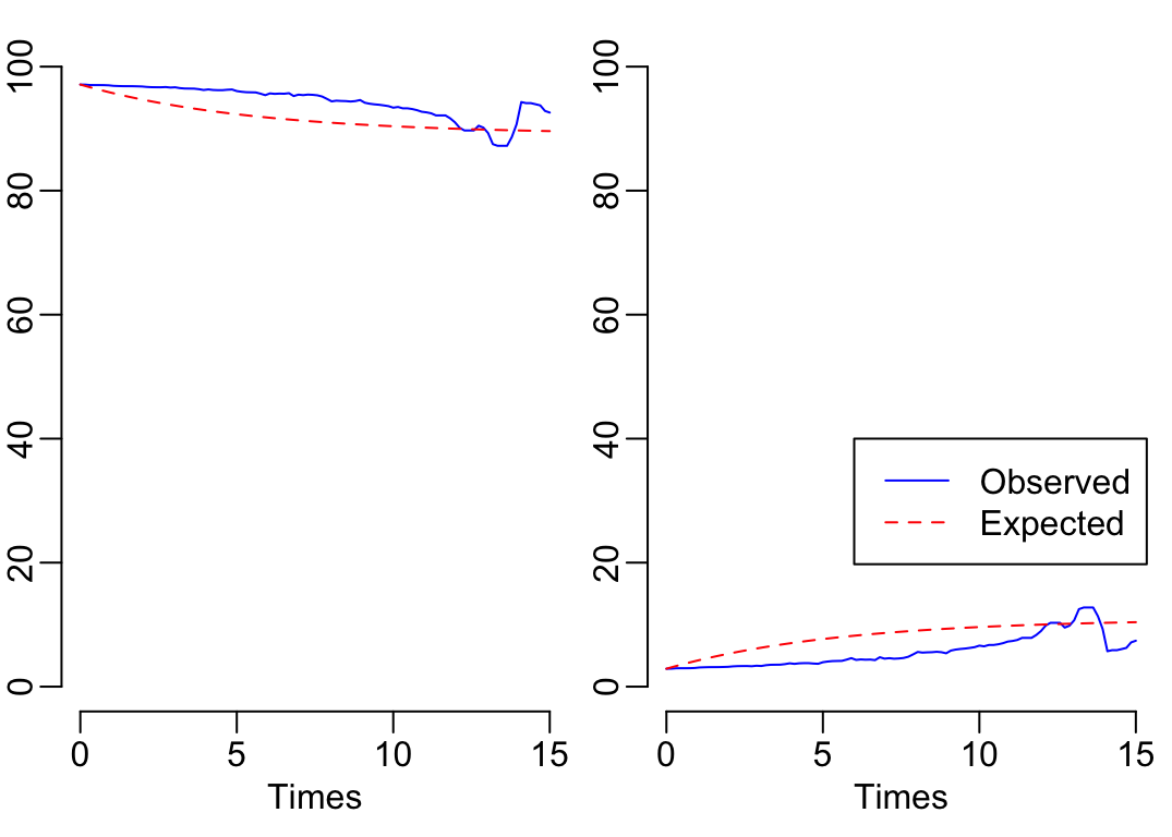
11 Pipelines
11.1 The pipelines
A first pipeline without any covariate:
pipeline1 <- function(bacteria) {
  if (bacteria == "all") bacteria <- bugs
  bacteria |>
    msm_data2() |>
    bsm(state ~ days, USUBJID, data = _) |>
    bsm_estimations() |>
    round(2)
}
Looking at the presence of other CRE at adminssion as a covariate:
pipeline2 <- function(bacteria) {
  if (bacteria == "all") bacteria <- bugs
  bacteria |>
    msm_data2() |>
    add_other_CRE_at_admission(bacteria) |>
    bsm(state ~ days, USUBJID, data = _, covariates = ~ otherCRE) |>
    HR()
}
Pipeline 3:
pipeline3 <- function(bacteria) {
  if (bacteria == "all") bacteria <- bugs
  bacteria |>
    msm_data2() |>
    add_ward() |>
    add_CRE_prevalence_in_ward() |>
    bsm(state ~ days, USUBJID, data = _, covariates = ~ estimate) |>
    HR()
}
Pipeline 4:
pipeline4 <- function(bacteria) {
  if (bacteria == "all") bacteria <- bugs
  bacteria |>
    msm_data2() |>
    add_ward() |>
    add_CRE_prevalence_in_ward() |>
    bsm(state ~ days, USUBJID, data = _, covariates = ~ lower) |>
    HR()
}
Pipeline 5:
pipeline5 <- function(bacteria) {
  if (bacteria == "all") bacteria <- bugs
  bacteria |>
    msm_data2() |>
    add_ward() |>
    add_CRE_prevalence_in_ward() |>
    bsm(state ~ days, USUBJID, data = _, covariates = ~ upper) |>
    HR()
}
11.2 Running pipelines
Let’s estimate the colonization and clearance rates for several different sets of bacteria:
bacteria_sets <- c("all", "Escherichia coli", "Klebsiella pneumoniae",
                   "Enterobacter hormaechei")
Estimates without any covariates (takes 10”):
pipeline1_results <- bacteria_sets |>
  set_names() |>
  map(pipeline1)
which gives:
pipeline1_results$all
estimate lower upper
colonization 9.73 8.54 11.10
clearance 10.09 8.06 12.63
$`Escherichia coli`
estimate lower upper
colonization 6.14 5.35 7.05
clearance 9.10 7.23 11.44
$`Klebsiella pneumoniae`
estimate lower upper
colonization 1.98 1.52 2.56
clearance 16.12 10.85 23.94
$`Enterobacter hormaechei`
estimate lower upper
colonization 2.42 0.92 6.36
clearance 76.11 26.64 217.46Testing the significativity of the presence of other CRE at admission as a covariate (takes 10”):
pipeline2_results <- bacteria_sets |>
  set_names() |>
  map(pipeline2)
which gives:
pipeline2_results$all
$all$otherCRETRUE
HR
State 1 - State 2 1
State 2 - State 1 1
$`Escherichia coli`
$`Escherichia coli`$otherCRETRUE
HR L U
State 1 - State 2 0.6458159 0.3147516 1.325102
State 2 - State 1 0.4730710 0.1951850 1.146585
$`Klebsiella pneumoniae`
$`Klebsiella pneumoniae`$otherCRETRUE
HR L U
State 1 - State 2 0.9110862 0.4757068 1.744936
State 2 - State 1 0.9151855 0.3995370 2.096338
$`Enterobacter hormaechei`
$`Enterobacter hormaechei`$otherCRETRUE
HR L U
State 1 - State 2 3.360957 0.2204102 51.25004
State 2 - State 1 3.964334 0.2635278 59.63676(takes 10”)
pipeline3_results <- bacteria_sets |>
  set_names() |>
  map(pipeline3)
which gives:
pipeline3_results$all
$all$estimate
HR L U
State 1 - State 2 2.0674313 0.53893895 7.930902
State 2 - State 1 0.2933742 0.03424017 2.513669
$`Escherichia coli`
$`Escherichia coli`$estimate
HR L U
State 1 - State 2 1.1283065 0.25865181 4.921967
State 2 - State 1 0.2915283 0.03355494 2.532824
$`Klebsiella pneumoniae`
$`Klebsiella pneumoniae`$estimate
HR L U
State 1 - State 2 0.22660676 0.015606843 3.290263
State 2 - State 1 0.04176564 0.001096988 1.590144
$`Enterobacter hormaechei`
$`Enterobacter hormaechei`$estimate
HR L U
State 1 - State 2 0.060099413 6.153152e-08 58700.639
State 2 - State 1 0.007279521 8.506564e-09 6229.476(takes 10”)
pipeline4_results <- bacteria_sets |>
  set_names() |>
  map(pipeline4)
which gives:
pipeline4_results$all
$all$lower
HR L U
State 1 - State 2 1.162162199 1.614677e-02 83.646526
State 2 - State 1 0.003858536 4.587443e-06 3.245446
$`Escherichia coli`
$`Escherichia coli`$lower
HR L U
State 1 - State 2 0.052651043 4.744167e-04 5.843244
State 2 - State 1 0.003802618 3.049806e-06 4.741252
$`Klebsiella pneumoniae`
$`Klebsiella pneumoniae`$lower
HR L U
State 1 - State 2 0.1272535347 4.829850e-05 335.27876
State 2 - State 1 0.0004029038 1.074142e-08 15.11266
$`Enterobacter hormaechei`
$`Enterobacter hormaechei`$lower
HR L U
State 1 - State 2 5.031146e-08 1.243504e-22 2.035573e+07
State 2 - State 1 2.435290e-13 3.273873e-28 1.811506e+02(takes 10”)
pipeline5_results <- bacteria_sets |>
  set_names() |>
  map(pipeline5)
which gives:
pipeline5_results$all
$all$upper
HR L U
State 1 - State 2 2.5665495 0.86330360 7.630197
State 2 - State 1 0.2206895 0.03858718 1.262177
$`Escherichia coli`
$`Escherichia coli`$upper
HR L U
State 1 - State 2 1.7425888 0.54849055 5.536314
State 2 - State 1 0.2831742 0.04920081 1.629803
$`Klebsiella pneumoniae`
$`Klebsiella pneumoniae`$upper
HR L U
State 1 - State 2 0.72878098 0.081375047 6.5268376
State 2 - State 1 0.02277722 0.001089422 0.4762178
$`Enterobacter hormaechei`
$`Enterobacter hormaechei`$upper
HR L U
State 1 - State 2 1119.746 12.48434 100432.4
State 2 - State 1 2739.253 17.33253 432914.812 Hierarchical model
Loading rstan:
library(rstan)Loading required package: StanHeaders
rstan version 2.32.7 (Stan version 2.32.2)For execution on a local, multicore CPU with excess RAM we recommend calling
options(mc.cores = parallel::detectCores()).
To avoid recompilation of unchanged Stan programs, we recommend calling
rstan_options(auto_write = TRUE)
For within-chain threading using `reduce_sum()` or `map_rect()` Stan functions,
change `threads_per_chain` option:
rstan_options(threads_per_chain = 1)
Attaching package: 'rstan'The following object is masked from 'package:tidyr':
extractThe following object is masked from 'package:magrittr':
extractrstan_options(auto_write = TRUE)
options(mc.cores = parallel::detectCores())Generating the province, hospital and ward data:
provinces <- setNames(rep(c("Dong Thap", "Phu Tho"), each = 6),
                      c("010", "008", "071", "073",
                        160, 161, 130, 155, 156, 157, 158, 159))

prov_hosp_ward <- CRF$ADM |>
  mutate(across(starts_with("WARD"), as.numeric),
         ward = paste0(SITEID, WARD_1, WARD_2, WARD_3)) |>
  arrange(SITEID) |>
  select(USUBJID, SITEID, ward) |>
  rename(hosp = SITEID) |>
  mutate(prov = provinces[hosp])
Preparing the data for K. pneumoniae:
tmp <- Kp_msm |>
  mutate(SampleSchedule = ifelse(days == 0, "admission", "discharge"))

durations <- tmp |>
  pivot_wider(id_cols = -state, names_from = SampleSchedule, values_from = days) |>
  select(-admission) |>
  rename(days = discharge)

adj_obs <- tmp |>
  pivot_wider(id_cols = -days, names_from = SampleSchedule, values_from = state) |>
  left_join(durations, "USUBJID") |>
  left_join(prov_hosp_ward, "USUBJID") |>
  select(USUBJID, prov, hosp, ward, admission, discharge, days)
#stan_data