Downscaling is a procedure that consists in infering high-resolution information from low-resolution data. This can be performed either in time or, more commonly, in space. Methodologically, it can be performed statistically (statistical downscaling) based on observed relationships between the variables of our data or mechanistically (often called dynamical downscaling), using a mechanistical model of the process generating the data. Such techniques are widely used for example in meteorology and climatology in order to derive local-scale weather and climate from Global Climate Models (GCM) data that have a typical resolution of 50 x 50 km. See for example the CORDEX project. Downscaling is not easy and, unfortunately, very few tools, if any, exist in R to for that (see for example this StackOverflow post). Here I use a very simple example of statistical temporal downscaling based on the use of linear models in order to illustrate what are the difficulties and when such methods can and shouldn’t be used.
Often downscaling is misunderstood as a problem of interpolation. Even
though there are common aspects of the two techniques, the problems of
interpolation and downscaling are radically different and downscaling is
substantially more difficult than interpolation. To illustrate this, let’s
consider a simple example using measures of temperature as a function of time.
Imagine that you measure temperature once per quarter, on the 15th of
February, the 15th of May, the 15th of August and the 15th of November. If
you want to infer the temperatures on the 15th of the other months from these
4 measures, you can use an interpolation technique which consist in fitting
these data to a model, either statistial such as a linear regression, or
mechanistical. For example, in base R, the function
approx()
allows to perform linear interpolation and the function
spline()
allows to perform spline interpolation. See the examples of these functions to
get a sense of what they are doing.
Let’s now imagine a slightly different situation: instead of having measures of temperatures at one time point per quarter, you have the average temperature per quarter and you would like, as before, to get an estimate of the temperature on the 15th of every month. Compared to the above situation of infering values at certain time points from values measured at other time points, here we want to infer values at certain time points from aggregates of values at other time points. Thus, instead of guessing values in between measured values, the problem here is to guess the values that where used to generate the aggregated values we have at hand. The type of aggregation could be the mean, as in our example, but it could be something else, cumulative sum for example. The figure below illustrates the differences between interpolation and downscaling.
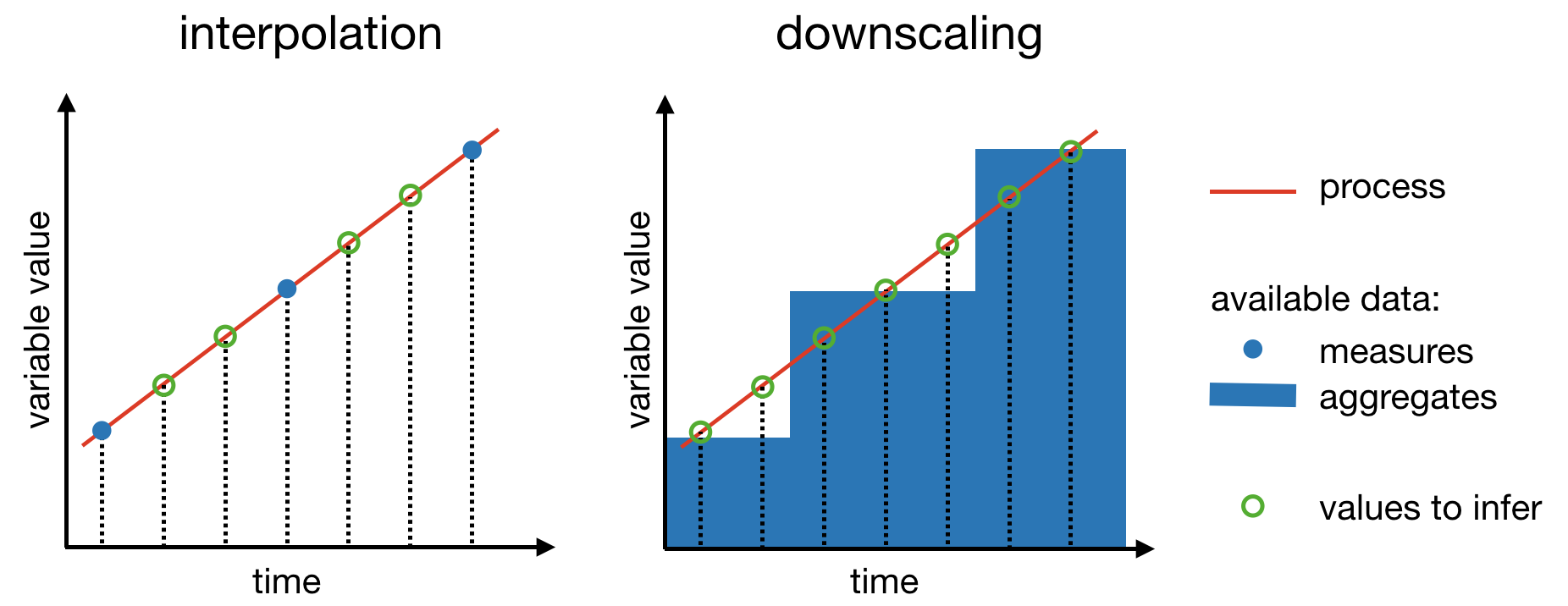
Whatever technique we use to perform downscaling, we generally want to comply to two constraints:
within each time interval, the aggregate of the infered values should be equal to the initial aggregate datum;
between all the time intervals, there should be a transition as smooth as possible.
Here, time intervals refers to the time intervals to which the initial aggregate data correspond, a quarter for example in our above example. In the case of spatial downscaling (2 dimensions instead of 1), we would probably speak of pixel instead of interval. These two constraints can be achieved easily with the use of linear models. More sophisticated methods such as spline would do better job but also be more complicated. For the purpose of illustrating the concepts, we will thus stick to the simplest method and we will assume that the aggregates are means (we’ll see that a cumulative sum won’t be much more difficult).
Step-by-step R code
We want to design a function that takes as inputs two vectors, one (y) of
aggregate values, the other one (x) being the time coordinates of the middle
of the time intervals to which the aggregates correspond. For the sake of
illustration we can consider the concrete example were we have the rates of
change of a population averaged by year and we want to downscale these data
so that we can express the rates of change of this population averaged by
semester. The first step consists in identifying the limits of the intervals to
which the aggregates correspond to, as materialized by the red vertical lines on
the figure below.
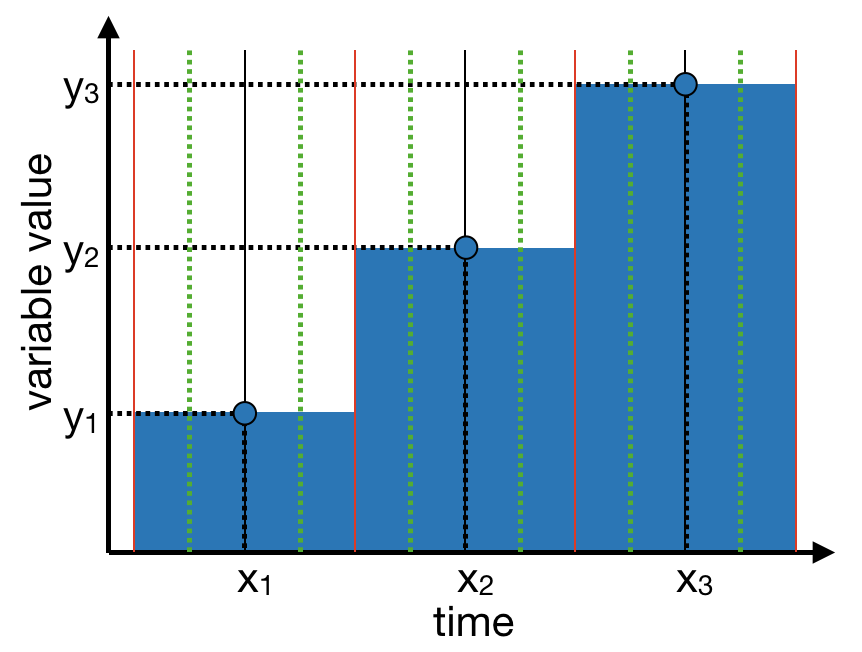
The function below, used with the option with_borders = TRUE, allows to do so:
centers <- function(x, with_borders = FALSE) {
  ctrs <- x[-1] - diff(x) / 2
  if (with_borders)
    return(c(2 * x[1] - ctrs[1], ctrs, 2 * tail(x, 1) - tail(ctrs, 1)))
  ctrs
}
To meet the first constraint, we simply need, on each of the intervals, to
define a linear model that goes through the blue dots of the above figure.
Furthermore, we know that through any two dots goes one and only one line. Thus,
the second contraint is easy to address too as long as we know, for each
interval, the y value of the linear model on the previous interval at the
limit between the two intervals (vertical red lines on the figure above). We can
thus design a recursive algorithm that estimates linear models for each
interval from left to right and the for-loop below does the job:
nb <- length(x)
the_centers <- centers(x, TRUE)
y2 <- c(y2_0, rep(NA, nb))
for(i in 1:nb) {
  x_val <- c(the_centers[i], x[i])
  y_val <- c(y2[i], y[i])
  m <- lm(y_val ~ x_val)
  y2[i + 1] <- predict(m, data.frame(x_val = the_centers[i + 1]))
}
where nb is the number of intervals and the_centers is an output of the
centers() function. The problem however concerns the first of these intervals
for which, by definition, we don’t have a previous interval and thus no left
point through which to make our linear model go through. Let’s call y2_0 the
y coordinate of this initial left point. In principle, we could choose any
value for y2_0. However, in order to meet our second constraint, let’s instead
consider applying an optimization algorithm in order to find the y2_0 that
makes the transitions between intervals as smooth as possible. For that, let’s
define unsmoothness as the sum of the absolute differences between the slopes
of adjacent linear models. The following function computes such a statistic from
a list of linear models:
unsmoothness <- function(list_of_models) {
  require(magrittr)
  list_of_models %>%
    sapply(get_slope) %>%
    diff() %>%
    abs() %>%
    sum()
}
where the function get_slope() would be defined by the following code:
get_slope <- function(model) coef(model)[2]What we need then to perform this optimization, is a function that takes a value
for y2_0 as an input and returns a list of models. The following function
built around the above for-loop does the job:
make_models <- function(y2_0) {
  models <- vector("list", nb)
  y2 <- c(y2_0, rep(NA, nb))
  for(i in 1:nb) {
    x_val <- c(the_centers[i], x[i])
    y_val <- c(y2[i], y[i])
    models[[i]] <- m <- lm(y_val ~ x_val)
    y2[i + 1] <- predict(m, data.frame(x_val = the_centers[i + 1]))
  }
  models
}
As we can see, this funtion returns a list of models that we can then feed to
unsmoothness() in order to find the value of unsmoothness that corresponds to our
choice of y2_0. And the combination of make_models() and unsmoothness() can
be used by the base R optimize() function in order to find the optimal value
of y2_0 over a given interval that minimize the unsmoothness. The problem
now is to define the interval to search in. An option could be given by the
following function:
range2 <- function(..., n = 1, na.rm = FALSE) {
  the_range <- range(..., na.rm = na.rm)
  n * c(-1, 1) * diff(the_range) / 2 + mean(the_range)
}
that is basically a wrapper around the base R function range() that allows to
reduce or expand the range. We can now look for the optimal value of y2_0 by
the following call:
optimize(function(x) unsmoothness(make_models(x)), range2(y, n = 3))$minimumOnce we have our optimal linear models on each of our intervals, the last step
consists in infering the new y values at a number of x values and this step
requires an additional little precaution in order to ensure that the first of
the two constraints listed above is met. Let’s call n the number of time
points per time interval at which we wish to infer y values. In case where we
want these points to be spread over each interval so that they represent the
middles of n equal-duration sub-intervals, the x coordinates of these points
can be computed by the following function:
subsegment_center <- function(x, n) {
  the_centers <- centers(x, TRUE)
  bys <- diff(the_centers) / n
  Map(seq, from = the_centers[seq_along(x)] + bys / 2, by = bys, le = n)
}
This function is basically a mapping of seq() on its parameters from and
by. Note that in the particular case where the initial x values are
regularly spaced, then all the values of the bys vector will be the same.
The final step will be a call to the predict() function in order to produce
the infered y values:
unlist(Map(predict,
           models,
           lapply(subsegment_center(x, n), function(x) data.frame(x_val = x))))
Note that the elements of the list outputed from make_new_x() are converted
into a data.frame in order to meet the requirement of the predict()
function.
Wrapping into one function
All the code above can be wrapped into one single function of three arguments:
y the data of aggregated values, x the centers of the (time) intervals to
which these aggregated values correspond, and n the number of new y values
we want to generate within each of these intervals:
downscale <- function(y, x, n) {
  require(magrittr)

  nb <- length(x)
  the_centers <- centers(x, TRUE)

# The function that makes the list of linear models (one per interval).
# Note that it uses `nb` and `the_centers` defined above.
  make_models <- function(y2_0) {
    models <- vector("list", nb)
    y2 <- c(y2_0, rep(NA, nb))
    for(i in 1:nb) {
      x_val <- c(the_centers[i], x[i])
      y_val <- c(y2[i], y[i])
      models[[i]] <- m <- lm(y_val ~ x_val)
      y2[i + 1] <- predict(m, data.frame(x_val = the_centers[i + 1]))
    }
    models
  }

# Using the function `unsmoothness()` to find the best `y2_0` value:
  best_y2_0 <- optimize(
    function(x) unsmoothness(make_models(x)),
    range2(y, n = 3)
  )$minimum

# Generating the list of models with the best `y2_0` value:
  models <- make_models(best_y2_0)

# Now that everything is ready:
  x %>%
    subsegment_center(n) %>%
    lapply(function(x) data.frame(x_val = x)) %>%
    Map(predict, models, .) %>%
    unlist()
}
Testing the function:
Let’s now test the function downscale(). Let’s consider 10 time intervals of
centers from 1 to 10 and let’s say we want to infer 12 values per interval:
x <- 1:10
n <- 12
The limits between these intervals are
the_centers <- centers(x, TRUE)And the x coordinates of the infered values will be
new_x <- unlist(subsegment_center(x, n))Let’s start with a simple example where the initial aggregate data are values from 1 to 10:
y1 <- 1:10
y1b <- downscale(y1, x, n)
plot(new_x, y1b)
points(x, y1, col = "blue", pch = 19)
abline(v = the_centers, col = "red")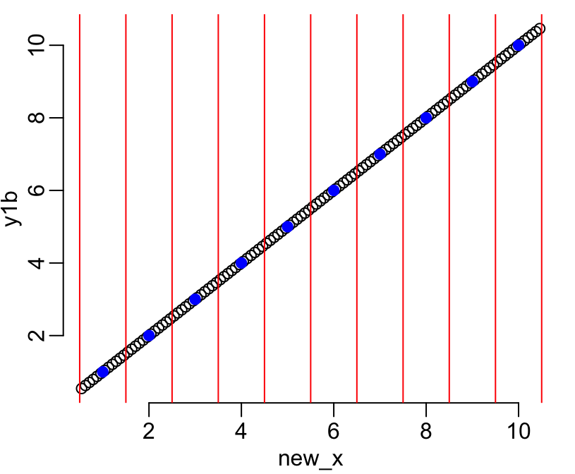
On this figure the vertical red lines show the limits of the intervals, the blue dots show the aggregated values available for each of these intervals, and the black dots show the infered disaggregated values within each interval. The figure shows that the continuity between intervals is respected (second of the above-listed constraints). Let’s now check that the first constraint is also well respected (i.e. that the aggregates of the infered values are equal to the initial aggregate data):
plot(y1, colMeans(matrix(y1b, n)),
     xlab = "initial aggregate data",
     ylab = "aggregates of infered values")
abline(0, 1)
That works fine! Let’s now consider a slightly more complicated example that
scrambles the values of y:
y2 <- sample(y1)
y2b <- downscale(y2, x, n)
plot(new_x, y2b)
points(x, y2, col = "blue", pch = 19)
abline(v = the_centers, col = "red")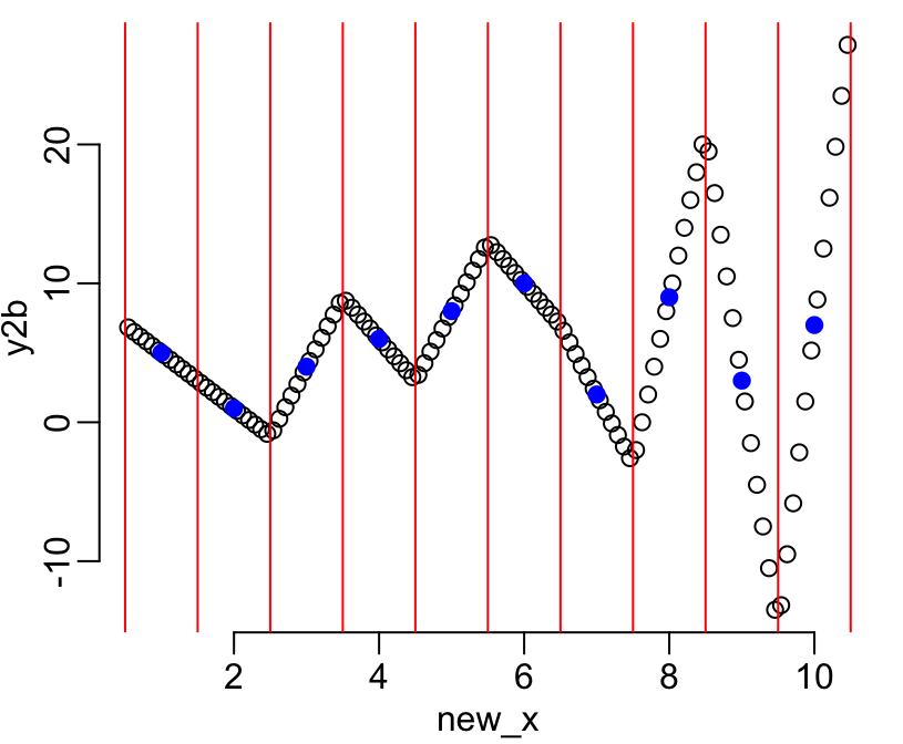
plot(y2, colMeans(matrix(y2b, n)),
     xlab = "initial aggregate data",
     ylab = "aggregates of infered values")
abline(0, 1)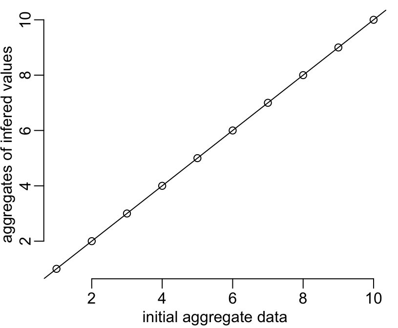
Works well too!
Conclusions
The function downscale() shows a very simple example of statistical
temporal (i.e. one dimension) downscaling, using linear models. This is
probably the simplest example of downscaling. This function could be
complexified in basically 2 non-incompatible directions: adding dimensions
(to consider spatial downscaling for example) and considering more complex
models. The latter can be done either by still considering statistical models
such as spline smoothing for example, or by considering mechanistical
(dynamical) models. The second option will provide a less general tool and will
require some domain knowledge. The functions centers(), range2(),
subsegment_center() and downscale() are available in the package
mcstats. To install it locally, just
type:
# install.packages("devtools")
devtools::install_github("choisy/mcstats")