Introduction
Packages
library(sp)
library(raster)
library(magrittr)
Simple mean
globcov <- globcoverVN::getgcvn()which gives
globcov## class : RasterLayer
## dimensions : 5339, 2636, 14073604 (nrow, ncol, ncell)
## resolution : 0.002777778, 0.002777778 (x, y)
## extent : 102.1458, 109.4681, 8.5625, 23.39306 (xmin, xmax, ymin, ymax)
## crs : +proj=longlat +datum=WGS84 +no_defs +ellps=WGS84 +towgs84=0,0,0
## source : /Library/Frameworks/R.framework/Versions/3.6/Resources/library/globcoverVN/extdata/globcoverVN.tif
## names : globcoverVN
## values : 11, 220 (min, max)WGS84 unprojected data.
plot(globcov)
Note that we can get access to the legend this way:
globcov@legend## An object of class ".RasterLegend"
## Slot "type":
## character(0)
##
## Slot "values":
## [1] 11 14 20 30 40 50 60 70 100 110 120 130 140 150 160 170 190
## [18] 200 210 220
##
## Slot "color":
## V1 V2 V3 V4 V5 V6 V7
## "#AAF0F0" "#FFFF64" "#DCF064" "#CDCD66" "#006400" "#00A000" "#AAC800"
## V8 V10 V11 V12 V13 V14 V15
## "#003C00" "#788200" "#8CA000" "#BE9600" "#966400" "#FFB432" "#FFEBAF"
## V16 V17 V19 V20 V21 V22
## "#00785A" "#009678" "#C31400" "#FFF5D7" "#0046C8" "#FFFFFF"
##
## Slot "names":
## [1] "Post-flooding or irrigated croplands (or aquatic)"
## [2] "Rainfed croplands"
## [3] "Mosaic cropland (50-70%) / vegetation (grassland/shrubland/forest) (20-50%)"
## [4] "Mosaic vegetation (grassland/shrubland/forest) (50-70%) / cropland (20-50%)"
## [5] "Closed to open (>15%) broadleaved evergreen or semi-deciduous forest (>5m)"
## [6] "Closed (>40%) broadleaved deciduous forest (>5m)"
## [7] "Open (15-40%) broadleaved deciduous forest/woodland (>5m)"
## [8] "Closed (>40%) needleleaved evergreen forest (>5m)"
## [9] "Closed to open (>15%) mixed broadleaved and needleleaved forest (>5m)"
## [10] "Mosaic forest or shrubland (50-70%) / grassland (20-50%)"
## [11] "Mosaic grassland (50-70%) / forest or shrubland (20-50%)"
## [12] "Closed to open (>15%) (broadleaved or needleleaved, evergreen or deciduous) shrubland (<5m)"
## [13] "Closed to open (>15%) herbaceous vegetation (grassland, savannas or lichens/mosses)"
## [14] "Sparse (<15%) vegetation"
## [15] "Closed to open (>15%) broadleaved forest regularly flooded (semi-permanently or temporarily) - Fresh or brackish water"
## [16] "Closed (>40%) broadleaved forest or shrubland permanently flooded - Saline or brackish water"
## [17] "Artificial surfaces and associated areas (Urban areas >50%)"
## [18] "Bare areas"
## [19] "Water bodies"
## [20] "Permanent snow and ice"
##
## Slot "colortable":
## logical(0)Next step now, in order to compute values of land cover per province, is to get the polygons of the provinces from GADM:
download.file("https://biogeo.ucdavis.edu/data/gadm3.6/Rsp/gadm36_VNM_1_sp.rds", "provinces.rds")Let’s load it:
provinces <- readRDS("provinces.rds")Which gives:
provinces## class : SpatialPolygonsDataFrame
## features : 63
## extent : 102.1446, 109.4692, 8.381355, 23.39269 (xmin, xmax, ymin, ymax)
## crs : +proj=longlat +datum=WGS84 +no_defs +ellps=WGS84 +towgs84=0,0,0
## variables : 10
## names : GID_0, NAME_0, GID_1, NAME_1, VARNAME_1, NL_NAME_1, TYPE_1, ENGTYPE_1, CC_1, HASC_1
## min values : VNM, Vietnam, VNM.1_1, An Giang, An Giang, NA, Thành phố , City, NA, VN.AG
## max values : VNM, Vietnam, VNM.9_1, Yên Bái, Yen Bai, NA, Tỉnh, Province, NA, VN.YBNote that the projection is the same as the raster. Let’s see what it looks like:
plot(globcov)
plot(provinces, add = TRUE)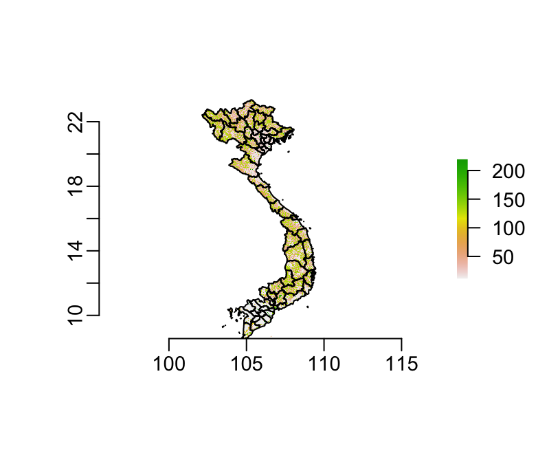
What we want to do now is, for each province, extracting the land cover data from the raster file that are inside the polygon of the province and then compute proportions. This is what the following function does:
proportion_lc <- function(x) {
  require(magrittr)
  prov <- provinces[x, ]
  rast <- crop(globcov, prov) # cropping before the mask
  mask(rast, rasterize(prov, rast)) %>%
    values() %>%
    na.exclude() %>%
    table() %>%
    {100 * . / sum(.)}
}
Note interestingly that, as noted here,
- a crop before the mask speeds up the masking by 6 and
- this
proportion_lc()function is about twice as fast as the use of theextract()function.
Let’s now compute this for all the provinces, which takes about 2’:
land_cover1 <- provinces %>%
  seq_along() %>%
  lapply(proportion_lc) %>%
  setNames(provinces@data$VARNAME_1) %>%
  c(., list(.id = "province")) %>%
  do.call(dplyr::bind_rows, .) %>%
  tidyr::replace_na(., as.list(setNames(rep(0, ncol(.)), names(.))))
Weighting by population densities
Now, let’s consider an alternative way of computing these propotions of land cover by province, weighting them by the local population density. We can retrieve the local population density for Vietnam as a raster file from WorldPop:
download.file("ftp://ftp.worldpop.org.uk/GIS/Population/Global_2000_2020/2010/VNM/vnm_ppp_2010.tif", "worldpop.tif")Let’s load it:
worldpop <- raster("worldpop.tif")It gives:
plot(worldpop)
plot(provinces, add = TRUE)
It also has the same projection than the other objects we’ve been dealing with so far:
worldpop## class : RasterLayer
## dimensions : 17796, 8789, 156409044 (nrow, ncol, ncell)
## resolution : 0.0008333333, 0.0008333333 (x, y)
## extent : 102.1454, 109.4696, 8.562917, 23.39292 (xmin, xmax, ymin, ymax)
## crs : +proj=longlat +datum=WGS84 +no_defs +ellps=WGS84 +towgs84=0,0,0
## source : /Users/choisy/Dropbox/aaa/www/blog/content/post/worldpop.tif
## names : worldpop
## values : 0.02010591, 568.1513 (min, max)However, it does not have the same resolution as globcov: there are about 10
times more pixels in worldpop than in globcov. Let’s thus resample
worldpop on globcov (takes about 2’):
worldpop2 <- resample(worldpop, globcov)We can check that it worked:
worldpop2## class : RasterLayer
## dimensions : 5339, 2636, 14073604 (nrow, ncol, ncell)
## resolution : 0.002777778, 0.002777778 (x, y)
## extent : 102.1458, 109.4681, 8.5625, 23.39306 (xmin, xmax, ymin, ymax)
## crs : +proj=longlat +datum=WGS84 +no_defs +ellps=WGS84 +towgs84=0,0,0
## source : memory
## names : worldpop
## values : 0.02054448, 558.3397 (min, max)and:
globcov## class : RasterLayer
## dimensions : 5339, 2636, 14073604 (nrow, ncol, ncell)
## resolution : 0.002777778, 0.002777778 (x, y)
## extent : 102.1458, 109.4681, 8.5625, 23.39306 (xmin, xmax, ymin, ymax)
## crs : +proj=longlat +datum=WGS84 +no_defs +ellps=WGS84 +towgs84=0,0,0
## source : /Library/Frameworks/R.framework/Versions/3.6/Resources/library/globcoverVN/extdata/globcoverVN.tif
## names : globcoverVN
## values : 11, 220 (min, max)Below is a new version of the proportion_lc() function that performs the
population weighting:
proportion_lc2 <- function(x) {
  require(magrittr)
  prov <- provinces[x, ]
  glcv <- crop(globcov, prov)
  wpop <- crop(worldpop2, prov)
  prov_mask <- rasterize(prov, glcv)
  glvc_val <- values(mask(glcv, prov_mask))
  wpop_val <- values(mask(wpop, prov_mask))
  weights <- wpop_val / sum(wpop_val, na.rm = TRUE)
  data.frame(glvc_val, weights) %>%
    na.exclude() %>%
    dplyr::group_by(glvc_val) %>%
    dplyr::summarize(val = sum(weights)) %$%
    setNames(val, glvc_val) %>%
    {100 * . / sum(.)}
}
Let’s apply it to all the provinces, it takes about 2’:
land_cover2 <- provinces %>%
  seq_along() %>%
  lapply(proportion_lc2) %>%
  setNames(provinces@data$VARNAME_1) %>%
  c(., list(.id = "province")) %>%
  do.call(dplyr::bind_rows, .) %>%
  tidyr::replace_na(., as.list(setNames(rep(0, ncol(.)), names(.))))
Let’s compare the 2 measures of land cover by province:
for (i in 2:ncol(land_cover1)) {
  x <- unlist(land_cover1[, i])
  y <- unlist(land_cover2[, i])
  xylim <- range(c(x, y))
  plot(y, x, xlim = xylim, ylim = xylim,
       xlab = "weighted by population density",
       ylab = "non weighted", col = "blue",
       main = globcov@legend@names[i - 1], cex.main = .5)
  abline(0, 1)
}


This figure shows clearly that the population tends to gather in the lower parts of the province.